Image filtering is one of the fundamental building blocks of computer vision. Whether you’re smoothing an image to remove noise or enhancing features for better detection, filtering techniques based on convolution are everywhere. In this article, we’ll explore image filtering using convolution — understanding the mathematics behind it, and seeing how it’s practically implemented in OpenCV. We’ll also cover popular filters like averaging, Gaussian blur, and custom kernels, all with sample code examples in Python and C++.

Import cv2

Before using any OpenCV functions, we must first import the library. This is the essential first step to access all OpenCV functionalities.

Python

# import the cv2 library
import cv2

C++

//Include Libraries
//OpenCV's cv::Mat acts like NumPy arrays for image processing.

#include<opencv2/opencv.hpp>
#include<iostream>

We are assuming  that you have already installed OpenCV on your device.
If not please refer the relevant links below:

• Install OpenCV on Windows
• Install OpenCV on MacOS
• Install OpenCV on Ubuntu

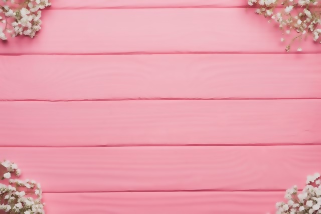
Example Image

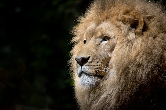
Image Filtering

At its core, image filtering involves modifying or enhancing an image by emphasizing certain features or suppressing others. This could mean:

• Smoothing to reduce noise
• Sharpening to enhance edges
• Edge detection to find object boundaries
• Embossing for stylistic effects

The common tool used for this purpose is convolution.

Convolution

Convolution is a mathematical operation that blends two functions together. In image processing, one function is the input image, and the other is a filter or kernel. Mathematically, in discrete form, convolution at a point (x,y)(x, y)(x,y) is defined as:

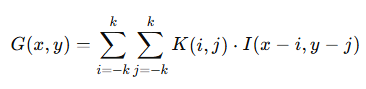
where:

• G(x,y)G(x, y)G(x,y) is the output pixel value at (x,y)(x, y)(x,y)
• I(x,y)I(x, y)I(x,y) is the input pixel value at (x,y)(x, y)(x,y)
• K(i,j)K(i, j)K(i,j) is the kernel value at (i,j)(i, j)(i,j)
• k defines the size of the kernel (for a (2k+1)×(2k+1) matrix)

Convolution involves sliding a kernel over each pixel of the image and computing the weighted sum of the pixel’s neighborhood. The result is a new transformed image.

Example of a 3×3 convolution kernel:

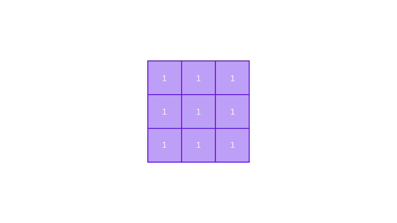
In simpler terms you move the small kernel matrix over the image, multiply overlapping values at the corresponding pixels, sum them up, and assign the result to the center pixel. This is why convolution is sometimes called a sliding window operation.

How to Use Kernels on Images

Filtering of a source image is achieved by convolving the kernel with the image. In simple terms, convolution of an image with a kernel represents a simple mathematical operation, between the kernel and its corresponding elements in the image.

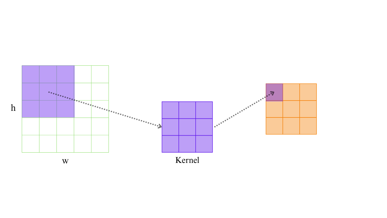
• Assume that the center of the kernel is positioned over a specific pixel (p), in an image.
• Then multiply the value of each element in the kernel (1 in this case), with the corresponding pixel element (i.e. its pixel intensity) in the source image.
• Now, sum the result of those multiplications and compute the average.
• Finally, replace the value of pixel (p), with the average value you just computed.

We perform this operation for every pixel in the source image, using the above 3×3 kernel, the resulting image will be a filtered image. You will soon see for yourself how the value of individual elements in a kernel dictate the nature of filtering. For example, by changing the value of the kernel elements, you can achieve different filtering effects. The concept is simple yet very powerful, and is therefore used in numerous image processing pipelines.

Now that you have learned to use convolution kernels, let’s explore how this is implemented in OpenCV for blurring and sharpening images.

Blurring An Image

Blurring, also known as smoothing, is a fundamental operation in image processing that aims to reduce the detail and noise in an image. It’s often used as a preprocessing step in tasks such as edge detection, object recognition, or even artistic effects like softening a photo. At its core, blurring is a convolution operation where each pixel in the output image is computed by taking a weighted average of the pixel and its neighboring pixels in the input image. This is done using a kernel (also called a filter or mask), which defines the weights of this averaging process.

Here’s a classic 3×3 average blurring kernel:

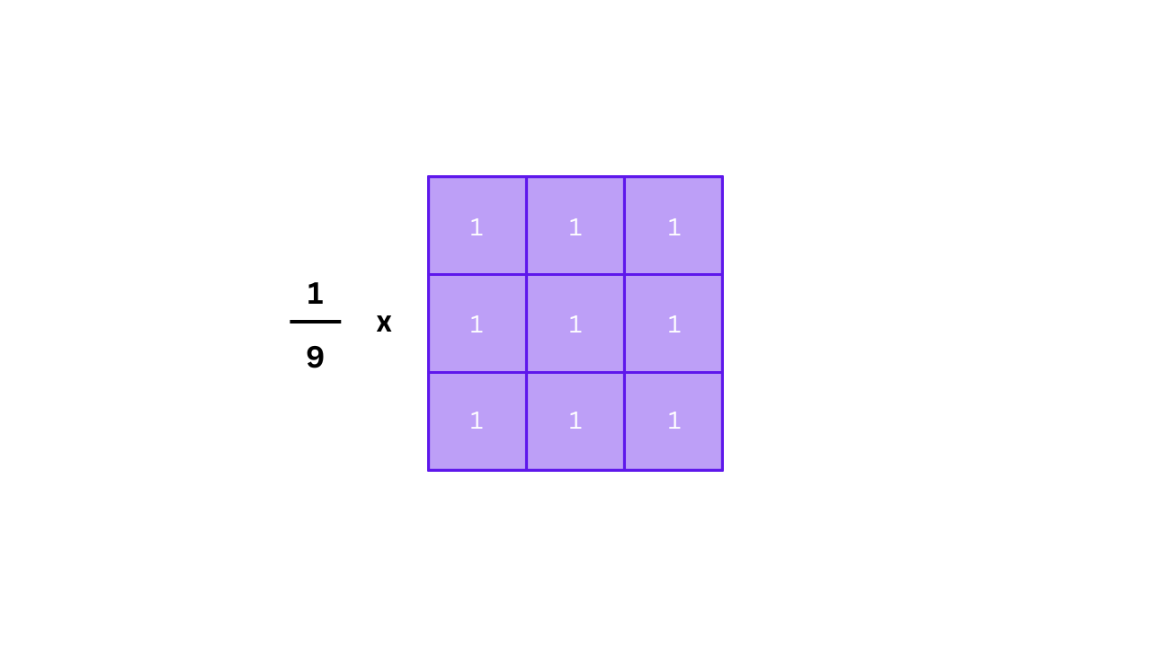
Here, each value in the kernel is the same — 1/9. This ensures that every pixel in the 3×3 neighborhood contributes equally to the result, and their total weight sums to 1.

The following steps occur:

1. Align the kernel over the first pixel: Place the center of the kernel pixel 1.
2. Multiply each kernel value by the corresponding pixel value in the image: For instance, the top-left kernel value (1/9) multiplies the top-left neighboring pixel intensity, and so on for all 9 elements.
3. Sum all the products: This sum is the weighted combination of the 9 pixels — effectively the average in this case.

0.11+0.44+0.66+0.22+0.44+0.77+0.55+0.33+0.22=3.74

4. Replace the original pixel value: The result from the above step becomes the new value of the first pixel in the output image.
   

This entire process is repeated for every pixel in the image (excluding borders, unless padding is used), so that each one is influenced by its neighbors. The result is an image that appears smoother because sharp intensity variations between adjacent pixels get softened.

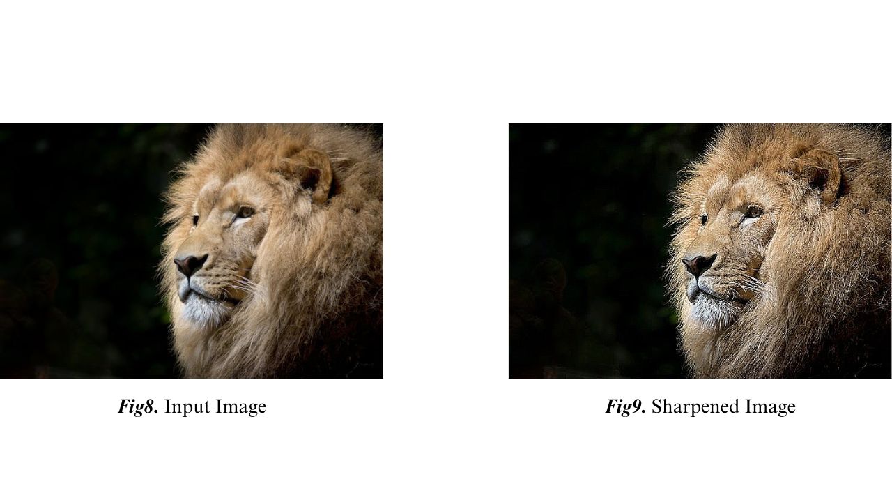
Sharpening an Image

If blurring is about softening an image by averaging neighboring pixels, then sharpening is its conceptual opposite. Sharpening enhances the edges and fine details in an image, making it appear crisper and more defined. It does this by emphasizing intensity transitions, particularly where pixel values change rapidly — the boundaries between objects, textures, or features.

Sharpening relies on highlighting the differences between a pixel and its surrounding neighbors. If a pixel’s value is significantly different from its neighbors, that means it’s likely on an edge or texture boundary — something we usually want to sharpen. If it’s similar to its neighbors, it’s likely in a flat, smooth area.

To achieve this, we use a convolution kernel that does two things simultaneously:

1. Preserves the center pixel with a positive weight.
2. Subtracts the influence of the surrounding pixels using negative weights.

Here’s a classic 3×3 sharpening kernel:

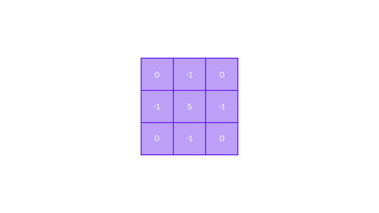
Center the kernel over the first pixel: The kernel aligns such that the center value (5) overlays the pixel 1, and the other values align with its 8 neighbors.

Multiply and sum:

• Multiply each kernel value with the corresponding pixel intensity beneath it.
• For neighbors, you’re subtracting their influence (because of the -1s).
• For the center, you’re increasing its contribution (5 times its value).

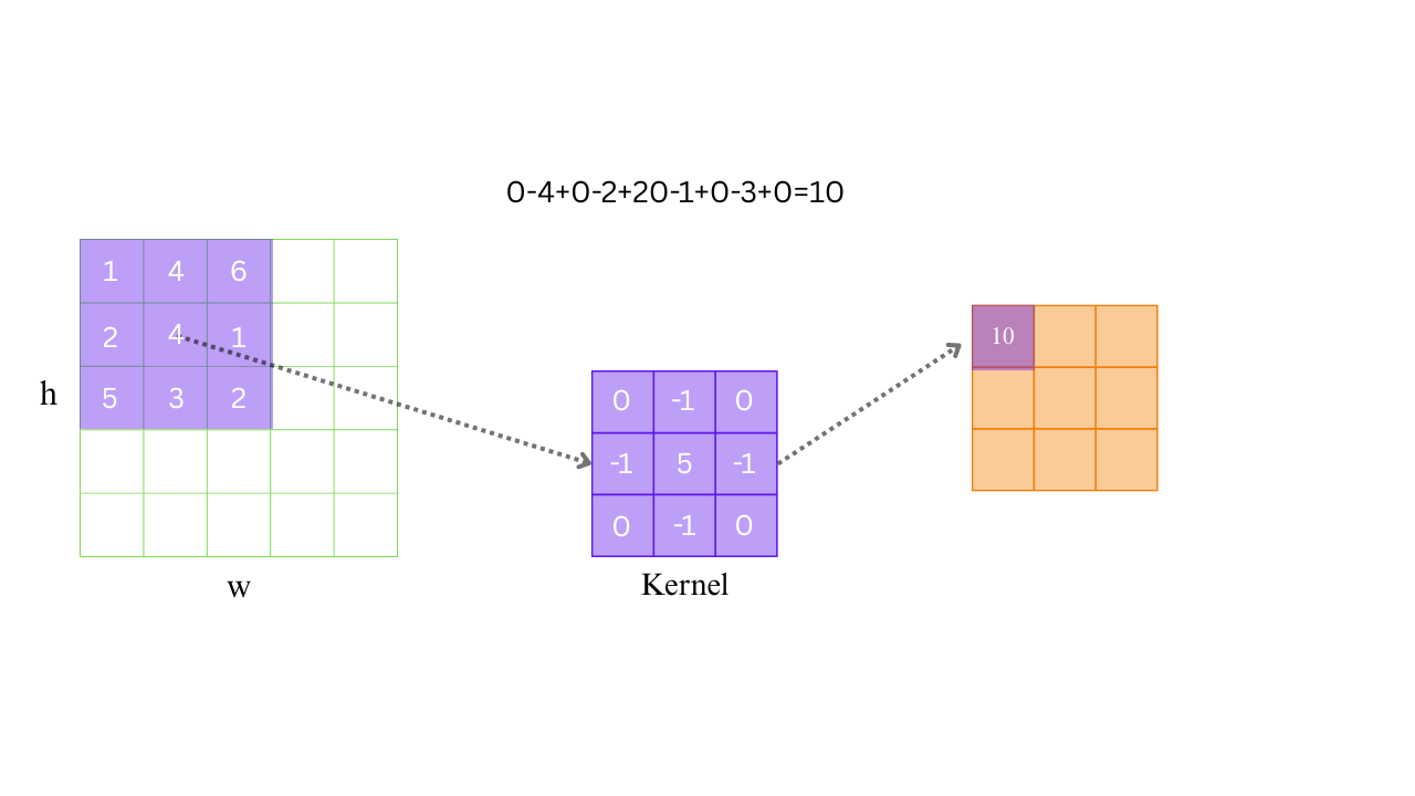
0-4+0-2+20-1+0-3+0=10

Update the pixel:

• The sum of these products becomes the new pixel value in the output image.
• The center pixel gets boosted, while surrounding pixels get subtracted — accentuating any contrast.

If the center pixel has a much higher value than its neighbors, the sharpened result becomes even higher, making the feature stand out more. If there is little contrast, the subtraction cancels out much of the center pixel’s influence — so flat areas stay flat.

Image Filtering using OpenCV

OpenCV provides powerful tools to perform filtering, ranging from flexible custom convolutions with filter2D() to optimized, ready-to-use functions for common effects like blurring and edge-preserving smoothing.

Custom Convolution

The most generic way to apply a filter to an image is by manually defining the kernel and using OpenCV’s filter2D() function. This function performs a 2D convolution between your image and a custom kernel.

Python

dst = cv2.filter2D(src, ddepth, kernel, anchor=(-1, -1), delta=0, borderType=cv2.BORDER_DEFAULT)

C++

cv::filter2D(src, dst, ddepth, kernel, anchor, delta, borderType);

Parameters:

• src: Input image (grayscale or color).
• dst: Output image (C++ only).
• ddepth: Desired depth of the output image. Use -1 to keep the same as input.
• kernel: A 2D array (usually np.float32 or cv::Mat) representing the filter.
• anchor: Position of the anchor point within the kernel (use (-1, -1) for center).
• delta: Optional value added to each pixel after filtering (used in some sharpening operations).
• borderType: Pixel extrapolation method at the border (e.g., cv2.BORDER_REFLECT, cv2.BORDER_CONSTANT).

We have implemented the 2D convolution for sharpening the image in the below section.

Built-in Filtering Functions

For standard operations like blurring and denoising, OpenCV provides several predefined filtering functions that internally perform optimized convolutions. These are easier to use and often more efficient than writing custom kernels manually.

Let’s explore the five most commonly used ones:

Generalized Averaging Filter-cv2.boxFilter()

The box filter applies a linear filter where each pixel in the output image is replaced with the average of its neighboring pixels within a defined kernel size. All kernel weights are equal.

Python:

dst = cv2.boxFilter(src, ddepth, ksize, normalize=True)

C++:

cv::boxFilter(src, dst, ddepth, ksize, anchor, normalize, borderType);

Parameters:

• ddepth: Output image depth. -1 to match input.
• ksize: Tuple or Size object like (5,5) defining the kernel size.
• normalize: If True, divide the result by the kernel area (default: True).
• anchor, borderType: Same as in filter2D().

Simplified Box Filter-cv2.blur()

This is a simpler wrapper over boxFilter() that always normalizes the result. It’s commonly used for mean blurring (basic smoothing).

Python

dst = cv2.blur(src, ksize)

C++

cv::blur(src, dst, ksize);

Parameters

• ksize: Size of the kernel, e.g., (3, 3).

Gaussian Weighted Blur-cv2.GaussianBlur()

This function applies a Gaussian kernel, which gives higher weight to the central pixels and lower to those further away. It produces a smoother, more natural blur compared to box blur.

Python

dst = cv2.GaussianBlur(src, ksize, sigmaX)

C++

cv::GaussianBlur(src, dst, ksize, sigmaX, sigmaY, borderType);

Parameters:

• ksize: Size of the Gaussian kernel (must be odd and positive).
• sigmaX: Standard deviation in the X direction.
• sigmaY: (Optional) If 0, it is computed from sigmaX.
• borderType: Optional border handling method.

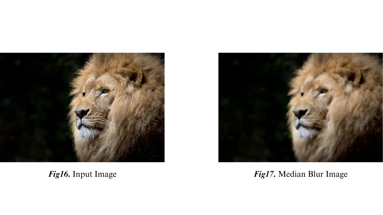
Non-Linear Median Filter-cv2.medianBlur()

Unlike the above filters, this applies a non-linear median operation. It replaces each pixel with the median value of its surrounding pixels. There is no fixed kernel matrix for median filtering.

Python

dst = cv2.medianBlur(src, ksize)

C++

cv::medianBlur(src, dst, ksize);

Parameters

• ksize: Aperture linear size. Must be an odd integer > 1.

Edge-Preserving Smoothing-cv2.bilateralFilter()

This filter smoothens flat regions while preserving edges. It considers both spatial distance and pixel intensity difference, making it one of the most advanced filters in OpenCV.

Like median blur, bilateral filtering does not use a fixed kernel matrix. It combines:

• Spatial Gaussian weights (based on distance from center pixel),
• Range Gaussian weights (based on intensity differences).

The actual kernel is computed dynamically for each pixel based on nearby values, so there’s no single static kernel.

Python

dst = cv2.bilateralFilter(src, d, sigmaColor, sigmaSpace)

C++

cv::bilateralFilter(src, dst, d, sigmaColor, sigmaSpace);

Parameters:

• d: Diameter of pixel neighborhood.
• sigmaColor: How dissimilar colors affect filtering (larger value = stronger smoothing).
• sigmaSpace: How far pixels influence each other spatially.

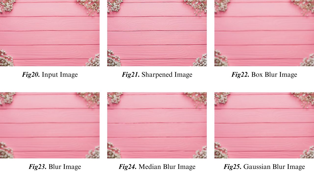
Implementation

Now that we’ve explored the theory and kernel structure behind each major filter, let’s implement them using OpenCV. In this section, we’ll apply the following filters:

1. Box Blur (cv2.blur / blur)
2. Gaussian Blur (cv2.GaussianBlur)
3. Median Blur (cv2.medianBlur)
4. Bilateral Filter (cv2.bilateralFilter)
5. Custom Sharpening Filter (cv2.filter2D with a sharpening kernel)

We’ll load an input image, apply all filters, display them, and save the results for comparison.

Python

import cv2
import numpy as np

# Load image
img = cv2.imread('blur3.jpg')
cv2.imshow('Original', img)

# 1. Box Filter using cv2.blur (simple averaging)
box1 = img.copy()
box = cv2.blur(box1, (7, 7))
cv2.imshow('Box Blur (cv2.blur)', box)
cv2.imwrite('box_blur.jpg', box)

# 1.1 Box Filter using cv2.boxFilter (more control)
box2 = img.copy()
box_filter = cv2.boxFilter(box2, -1, (7, 7), normalize=True)
cv2.imshow('Box Filter (cv2.boxFilter)', box_filter)
cv2.imwrite('box_filter.jpg', box_filter)

# 2. Gaussian Blur
guass = img.copy()
gaussian = cv2.GaussianBlur(guass, (7, 7), 0)
cv2.imshow('Gaussian Blur', gaussian)
cv2.imwrite('gaussian_blur.jpg', gaussian)

# 3. Median Blur
med = img.copy()
median = cv2.medianBlur(med, 7)
cv2.imshow('Median Blur', median)
cv2.imwrite('median_blur.jpg', median)

# 4. Bilateral Filter
bil = img.copy()
bilateral = cv2.bilateralFilter(bil, 9, 75, 75)
cv2.imshow('Bilateral Filter', bilateral)
cv2.imwrite('bilateral_blur.jpg', bilateral)

# 5. Custom Sharpening Filter
cus = img.copy()
kernel = np.array([[0, -1, 0],
                   [-1, 5, -1],
                   [0, -1, 0]])
sharpened = cv2.filter2D(cus, -1, kernel)
cv2.imshow('Sharpened', sharpened)
cv2.imwrite('sharpened.jpg', sharpened)

cv2.waitKey(0)
cv2.destroyAllWindows()

C++

#include <opencv2/opencv.hpp>
int main() {

    // Load image
    cv::Mat img = cv::imread("blur3.jpg");
    if (img.empty()) {
        std::cerr << "Could not open image!\n";
        return -1;
    }
    cv::imshow("Original", img);

    // 1. Box Blur using cv::blur
    cv::Mat box;
    cv::blur(img, box, cv::Size(7, 7));
    cv::imshow("Box Blur (cv::blur)", box);
    cv::imwrite("box_blur.jpg", box);

    // 1.1 Box Filter using cv::boxFilter
    cv::Mat boxFilter;
    cv::boxFilter(img, boxFilter, -1, cv::Size(7, 7), cv::Point(-1, -1), true, cv::BORDER_DEFAULT);
    cv::imshow("Box Filter (cv::boxFilter)", boxFilter);
    cv::imwrite("box_filter.jpg", boxFilter);

    // 2. Gaussian Blur
    cv::Mat gaussian;
    cv::GaussianBlur(img, gaussian, cv::Size(7, 7), 0);
    cv::imshow("Gaussian Blur", gaussian);
    cv::imwrite("gaussian_blur.jpg", gaussian);

    // 3. Median Blur
    cv::Mat median;
    cv::medianBlur(img, median, 7);
    cv::imshow("Median Blur", median);
    cv::imwrite("median_blur.jpg", median);

    // 4. Bilateral Filter
    cv::Mat bilateral;
    cv::bilateralFilter(img, bilateral, 9, 75, 75);
    cv::imshow("Bilateral Filter", bilateral);
    cv::imwrite("bilateral_blur.jpg", bilateral);

    // 5. Custom Sharpening using filter2D
    cv::Mat sharpened;
    cv::Mat kernel = (cv::Mat_<float>(3,3) <<
                       0, -1, 0,
                      -1, 5, -1,
                       0, -1, 0);
    cv::filter2D(img, sharpened, -1, kernel);
    cv::imshow("Sharpened", sharpened);
    cv::imwrite("sharpened.jpg", sharpened);

    cv::waitKey(0);
    cv::destroyAllWindows();
    return 0;
}

Explanation

We have used larger kernel sizes and higher values since the image is of higher resolution.

• cv2.blur(): Applies a normalized box filter; smooths the image by averaging pixel intensities over a neighborhood.
• cv2.boxFilter() gives you the option to set normalize=False, which lets you apply non-averaging box filters, e.g., for summation or custom behavior.
• cv2.GaussianBlur(): Uses a weighted kernel based on the Gaussian distribution. Smoother and more natural blurring effect, especially near edges.
• cv2.medianBlur(): Replaces each pixel with the median of its neighbors. Very effective against salt-and-pepper noise.
• cv2.bilateralFilter(): Performs blurring while preserving edges. Considers both spatial and intensity differences.
• cv2.filter2D() with a sharpening kernel: Enhances edges by subtracting neighboring pixel influence and boosting the center pixel.

Each filtered image is both displayed in a window and saved to disk, making it easy to compare the effects visually.

Output

Another Example Image

Summary

In this article, we explored image filtering using OpenCV, focusing on both custom and built-in filtering methods that rely on the powerful concept of convolution. Convolution works by applying a kernel (filter) over each pixel in the image, transforming it based on its local neighborhood.