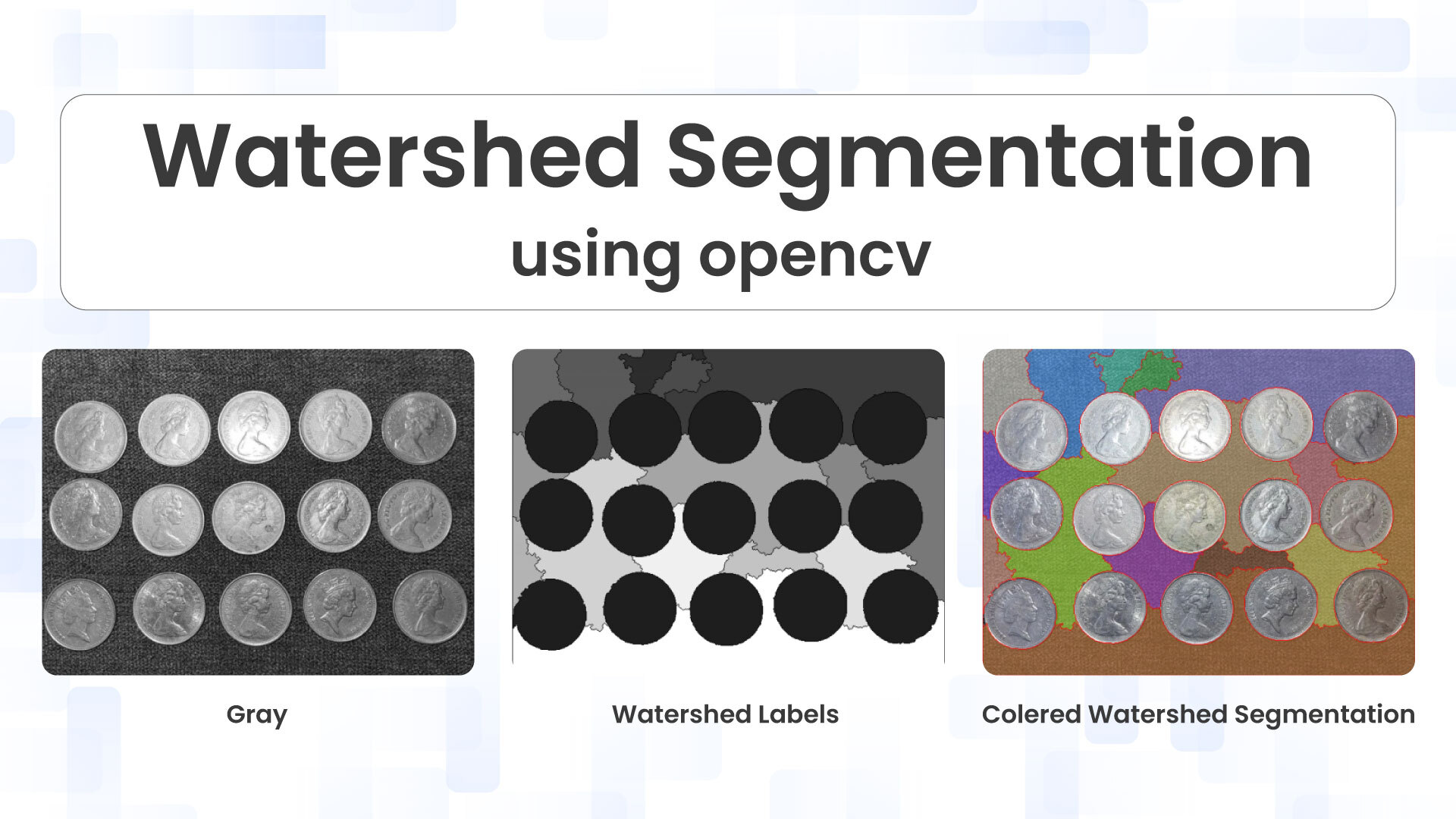
Counting overlapping or touching objects in images is a common challenge in computer vision. Simple thresholding and contour detection often fail when objects are in contact, treating multiple items as a single blob. The Watershed algorithm provides a solution to this problem by treating the image as a topographic surface and “flooding” it to separate touching objects.
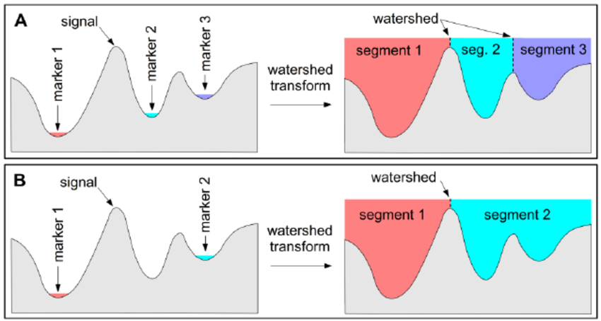
Table of contents
- Introduction to Watershed Algorithm
- Understanding the Watershed Algorithm: The Topographic Analogy
- Marker-Based Watershed: Overcoming Oversegmentation
- Understanding the Code: Step-by-Step
- Practical Tips and Common Pitfalls
- Real-World Applications of Watershed Segmentation
- Advanced Enhancements and Alternatives
- Conclusion and Further Learning Resources
- Essential Learning Resources
Introduction to Watershed Algorithm
Image segmentation is a cornerstone of modern computer vision, transforming raw pixel data into meaningful, analyzable regions. By partitioning an image into distinct segments, we enable machines to understand visual content at a semantic level, facilitating everything from medical diagnosis to autonomous vehicle navigation.
The watershed algorithm stands out amongst segmentation techniques for its exceptional ability to separate touching or overlapping objects, a challenge that often defeats simpler methods. Named after the geographic concept of drainage basins, this algorithm treats grayscale intensities as topographic elevations, creating natural boundaries where different regions meet.
Understanding the Watershed Algorithm: The Topographic Analogy
At its heart, the watershed algorithm employs a beautifully intuitive metaphor: imagine your grayscale image as a three-dimensional topographic landscape. Each pixel’s intensity value represents elevation-bright regions form peaks and ridges, while dark areas create valleys and basins. This transformation from a two-dimensional pixel grid to a three-dimensional terrain is the conceptual foundation that makes watershed segmentation so powerful and elegant.
Topographic Interpretation: The grayscale image becomes a landscape where high-intensity pixels form peaks and low-intensity pixels create valleys
Valley Flooding Process: Water floods the valleys from local minima, each source producing distinctly colored water representing different regions.
Barrier Construction : When waters from different basins meet, barriers are erected at these watershed lines, defining precise object boundaries.
The Oversegmentation Challenge:
Classical watershed implementations often suffer from oversegmentation, where minor noise and intensity irregularities create unwanted local minima. This results in an image divided into far too many tiny regions rather than meaningful objects. The marker-based approach we’ll explore next provides the elegant solution to this fundamental limitation.
Marker-Based Watershed: Overcoming Oversegmentation
The marker-based watershed approach revolutionises the classical algorithm by introducing human guidance or algorithmic intelligence into the segmentation process. Rather than allowing the algorithm to identify every possible local minimum as a starting point for flooding, we explicitly define markers that indicate sure foreground objects, definite background regions, and uncertain areas requiring algorithmic decision-making.
Sure Foreground: Regions we confidently identify as belonging to objects of interest, labelled with distinct positive integers.
Sure Background: Areas we know with certainty belong to the background, typically labelled as zero or a specific background marker.
Unknown Regions: Uncertain boundary zones where the algorithm must determine object membership, marked with zero values.
Understanding the Code: Step-by-Step
Let us break down the implementation into steps.
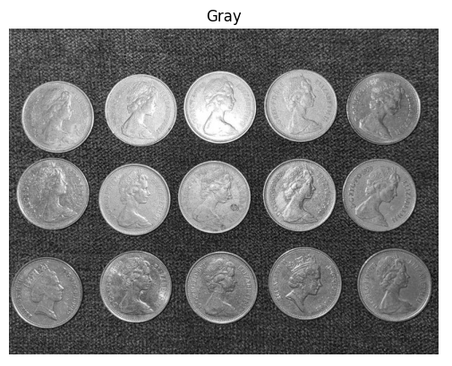
Step 1: Image Preprocessing
img = cv2.imread("coins.jpg")
img_rgb = cv2.cvtColor(img, cv2.COLOR_BGR2RGB)
gray = cv2.cvtColor(img, cv2.COLOR_BGR2GRAY)
We start by loading the image and converting it into grayscale. The watershed algorithm works on color images for the final segmentation, but we need grayscale for preprocessing.
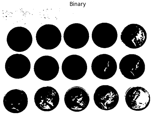
Step 2: Binary Thresholding
blur = cv2.GaussianBlur(gray, (5, 5), 0)
_, binary = cv2.threshold(blur, 0, 255, cv2.THRESH_BINARY_INV + cv2.THRESH_OTSU)
Here’s what happens:
- Gaussian blur reduces noise that could interfere with thresholding.
- Otsu’s thresholding automatically finds the optimal threshold value to separate foreground (coins) from background
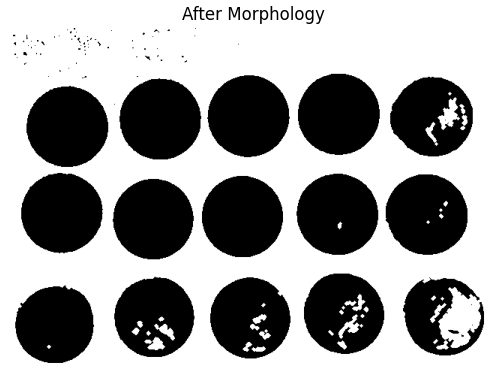
Step 3: Morphological Operations (Noise Removal)
kernel = cv2.getStructuringElement(cv2.MORPH_ELLIPSE, (3, 3))
opening = cv2.morphologyEx(binary, cv2.MORPH_OPEN, kernel, iterations=2)
Morphological opening (erosion followed by dilation) removes small noise and smooths object boundaries. This step is crucial because noise can create false markers and incorrect segmentation.
Step 4: Identifying Sure Background
sure_bg = cv2.dilate(opening, kernel, iterations=3)
We dilate the cleaned binary image to expand object regions. Everything in this dilated image is definitely either object or background. This becomes our “sure background” area.
Step 5: Distance Transform and Sure Foreground
dist = cv2.distanceTransform(opening, cv2.DIST_L2, 5)
_, sure_fg = cv2.threshold(dist, 0.35 * dist.max(), 255, 0)
sure_fg = np.uint8(sure_fg)
The distance transform is key to watershed segmentation:
- It calculates the distance of each white pixel to the nearest black pixel
- Pixels at object centers have the highest distances (they’re furthest from edges)
- By thresholding at 35% of the maximum distance, we identify regions that are definitely part of object centers
Step 6: Identifying Unknown Region
unknown = cv2.subtract(sure_bg, sure_fg)
The unknown region is the area between sure foreground and sure background. This is where touching coins overlap and where the watershed algorithm will determine the precise boundaries.
Step 7: Marker Labeling


num_labels, markers = cv2.connectedComponents(sure_fg)
markers = markers + 1
markers[unknown == 255] = 0
We use connected components to label each sure foreground region with a unique ID:
- Each coin center gets a distinct label (1, 2, 3, etc.)
- We add 1 to all labels so background becomes 1 instead of 0
- Unknown regions are set to 0 (these will be determined by watershed)
This labeling tells the watershed algorithm where each object is located.
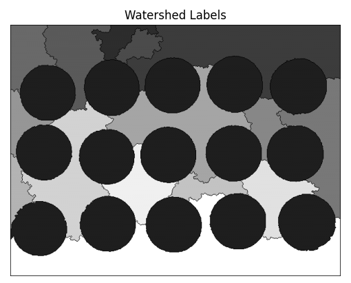
Step 8: Apply Watershed Algorithm
markers_ws = cv2.watershed(img, markers)
This is where the magic happens! The watershed algorithm:
- Takes the original color image and the marker labels
- “Floods” from each labeled region
- Creates boundaries (marked as -1) where different regions meet
- Returns an updated marker image with all pixels labeled
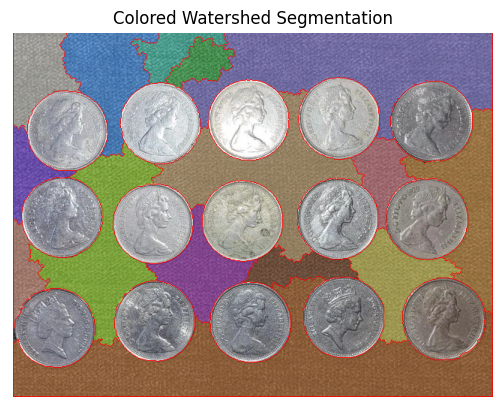
Step 9: Visualization and Counting
label_ids = np.unique(markers_ws)
label_ids = label_ids[label_ids > 1]
coin_count = len(label_ids[label_ids > 1])
We count the unique labels (excluding background and boundaries) to get the total number of coins. Each label represents one segmented coin.
For visualization, we assign random colors to each labeled region and overlay them on the original image, with watershed boundaries highlighted in red.
Key Parameters to Tune
When applying watershed to your own images, consider adjusting:
- Gaussian blur kernel size (5, 5): Larger values for noisier images
- Morphology kernel size (3, 3): Larger for bigger objects
- Distance transform threshold (0.35): Lower values detect more objects but may oversegment; higher values may undersegment
- Dilation iterations (3): Affects background region size
Practical Tips and Common Pitfalls
Mastering watershed segmentation requires understanding not just the algorithm’s mechanics, but also the subtle art of parameter selection and preprocessing optimisation. Even experienced practitioners encounter challenges when applying watershed to new image types or challenging lighting conditions. This section distils hard-won lessons into actionable guidance that will accelerate your journey from novice to expert.
Real-World Applications of Watershed Segmentation
Watershed segmentation’s unique ability to separate touching objects makes it invaluable across numerous industries and research domains. From life-saving medical diagnostics to industrial quality control, this algorithm solves practical problems where traditional segmentation methods fail. Understanding these applications provides context for implementation decisions and reveals optimization opportunities specific to your domain.
Medical Image Analysis: Cell counting and separation in microscopy images represents watershed’s flagship medical application. Pathologists use watershed-based tools to analyse blood smears, identify tumour cells, and quantify cellular features.
Industrial Quality Control: Manufacturing facilities deploy watershed segmentation for real-time defect detection and object counting on production lines.
Crowd Analysis and Tracking: Surveillance and crowd monitoring systems leverage watershed segmentation to identify and count individuals in densely packed scenes.
Document Analysis: Optical character recognition (OCR) systems employ watershed segmentation to separate touching characters in scanned documents, particularly crucial for handwritten text where letters frequently connect.
Advanced Enhancements and Alternatives
Whilst watershed segmentation provides robust results for many scenarios, cutting-edge applications often require combining watershed with complementary techniques or considering alternative approaches. Understanding the broader segmentation landscape empowers you to select the optimal method for your specific requirements, whether prioritising accuracy, speed, automation level, or ease of implementation.
Edge-Enhanced Watershed: Combining watershed with edge detection methods like Canny creates hybrid approaches that leverage both intensity gradients and edge information.
Machine Learning Marker Generation: Traditional marker-based watershed relies on hand-crafted rules for marker placement. Modern implementations replace this with learned approaches—train a classifier or neural network to predict optimal marker locations based on image features.
Hierarchical Watershed: Multi-scale watershed implementations process images at multiple resolutions, combining results to achieve robust segmentation across object sizes
Alternative Segmentation Methods
Several powerful alternatives deserve consideration depending on your application requirements. K-means clustering offers simpler implementation and faster processing but struggles with touching objects. GrabCut provides interactive segmentation with minimal user input, ideal for scenarios requiring human guidance. Deep learning approaches like U-Net deliver state-of-the-art accuracy on complex images but require substantial training data and computational resources.
Conclusion and Further Learning Resources
Watershed segmentation stands as a testament to the power of nature-inspired algorithms in computer vision. By drawing inspiration from the way water floods topographic landscapes, this technique transforms a simple physical analogy into a robust mathematical framework. As a result, it effectively addresses one of image analysis’s most persistent challenges, separating touching or overlapping objects. Throughout this technical journey, we have progressively moved from fundamental theory to practical implementation and, ultimately, to advanced applications. In doing so, this guide equips you with both a strong conceptual understanding and hands-on coding skills needed to apply watershed segmentation confidently in real-world scenarios.
Key Takeaways
- Watershed treats intensity as topography, creating natural object boundaries.
- Marker-based approaches overcome classical oversegmentation limitations.
- OpenCV provides robust, production-ready watershed implementation.
- Parameter tuning balances noise removal, marker conservatism, and accuracy.
- Integration with modern AI techniques unlocks cutting-edge capabilities.
Essential Learning Resources
- Official OpenCV Watershed Tutorial — comprehensive documentation with examples
- PyImageSearch Watershed Guide — detailed walkthrough with practical tips
- Scikit-image Watershed Examples — alternative Python implementation
- OpenCV GitHub Repository — sample code and test images


5K+ Learners
Join Free VLM Bootcamp3 Hours of Learning