---

Image retrieval is a long-standing computer vision problem. It is used in image indexing, e.g. Google’s image search. It is also used as the starting piece in many visual localisation methods.

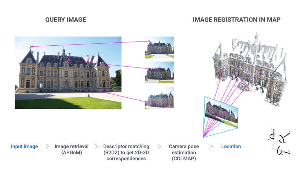
My favourite analogy is as follows: imagine you have a random piece of jigsaw puzzle which belongs to a hundred sets of puzzle boards – the goal of visual localisation is to fit that puzzle piece (pose of the query image) into the right location, while image retrieval is the first step of identifying which set out of those hundred quiz boards this piece actually belongs to.
In this blogpost I would first go through recent advances in deep image retrieval. Also, I would talk about my latest work in using second-order information with self-attention to improve these techniques, and how to visualise the results interactively with OpenCV. Hope you will find it helpful!

The Two Main Types of Deep Image Retrieval Techniques

In order to retrieve images, we have to compute the similarity between images. To efficiently rank the similarities between a large number of images, we first have to represent each image with a single vector, which is called a global descriptor. Think about how you can quite easily identify if two human faces are the same person without giving a second thought, even if you’ve never seen these faces before? This is your brain’s innate ability to ‘describe’ faces without having to analyse each and every detail of the faces. The global descriptor is in a sense very similar to this, as its name suggests, describing the image in a compressed manner. As a matter of fact, it was this famous face recognition paper that shot the triplet loss to fame, which is used by practically all image retrieval methods nowadays!

• 

---

Before the rise of the popularity of Deep Learning, image retrieval was mostly local feature-based. Local features, or local descriptors, similar to global descriptors, represent images with a vector. However, local descriptors only describe a small region of the image, which is called a patch. As early works in image description were mainly focused on local descriptors, such as the famous SIFT, they produced the global descriptor by aggregating these local descriptors, e.g. Bag of Words. 

As Deep Learning became more prevalent, learnt local features were also aggregated to form much more robust global descriptors, pioneered by Arandjelović et al. and Noh et al.’s works. We call such methods local aggregation.

Another consequence of Deep Learning to image retrieval is a different class of global descriptors which we call global single-pass. These descriptors rely on pooling feature maps from popular Convolutional Neural Networks (CNNs), such as AlexNet, VGG, ResNet etc. This is essentially analogous to aggregating local features, but using much more simple mathematical operations (such as max, median and mean) and is more widely supported by GPU accelerators. Therefore, global single-pass methods are more scalable (but often at the cost of accuracy and precision) and is the main focus of this blog post.

Recent Advances in Global Single-Pass Descriptors

With the success of CNNs supported by large amounts of training data, the image retrieval community began to realise the potential of CNN feature maps. Early attempts at aggregating features maps in a global descriptor, i.e. global-pooling, included Max-pooling, average-pooling. However, these features were from CNNs pre-trained on ImageNet, a dataset designed for image classification rather than image retrieval. Radenović et al.’s paper is a breakthrough in deep image retrieval as it not only introduced a dataset specific for ranking losses to fine-tune CNNs for image retrieval, it also presented a much more powerful pooling operation – GeM pooling.

This paper is very important to my research as it is not only the state-of-the-art method at the time, it is also one of the most comprehensive papers in image retrieval, which includes a huge amount of experiments and results, giving very clear hints in which directions subsequent researchers who are interested in the field should head towards. Moreover, their code is also extremely well written (800+ stars on GitHub) and my own code is heavily based on the framework they established, which includes all the models, datasets training and evaluation scripts required to reproduce results in the paper. It definitely saved me months worth of time! If you are interested in image retrieval, I highly suggest that you check their repository out.

If we have an input image I $ \in$ IR^{H, W,} з , after passing it through a CNN we get a feature map f = $\Theta$ (I) $ \in$ IR^{h, w, d} .

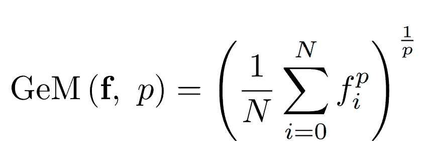
The GeM-pooling operation is
where N is the total number of features i.e. N = h x w.

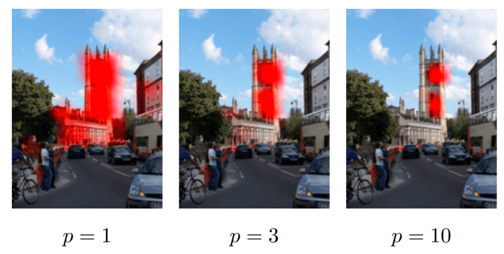
The formula might look intimidating but it is actually very intuitive! In simple terms, GeM takes the weighted-average of features in feature map f, and the weights are determined by the CNN’s activation of each feature. Therefore, the more reactive the CNN is to a feature, the more a feature contributes to the global descriptor. The scalar p then controls how much such weighting is skewed towards these “strong” features.

Second-Order Information in Pooling

For place recognition and visual localisation, image retrieval has to work well on landmark images. Landmark images present a few unique challenges compared to other domains. For example, looking at Figure 3., (a) different landmarks can look both very different or similar, (b) there can be multiple landmarks in one image, (c) most of the image is irrelevant or (d) the images can be taken in extreme conditions.

The limitation of GeM pooling is that each feature contains information only from around its spatial neighborhood, as it is a first-order measure. Using (b) Figure 3 as an illustration, how does GeM know whether the dome or the spire is more important? Or both? Therefore, we need something beyond first-order statistics to achieve a more robust global descriptor for landmarks.

Self-attention is an incredibly successful mechanism in utilising second-order information in Natural Language Processing’s Transformers and is very popular among various computer vision tasks as well. Figure 5 shows how it works. It might look very complex at first sight, but it’s actually quite simple! The steps are as follows:

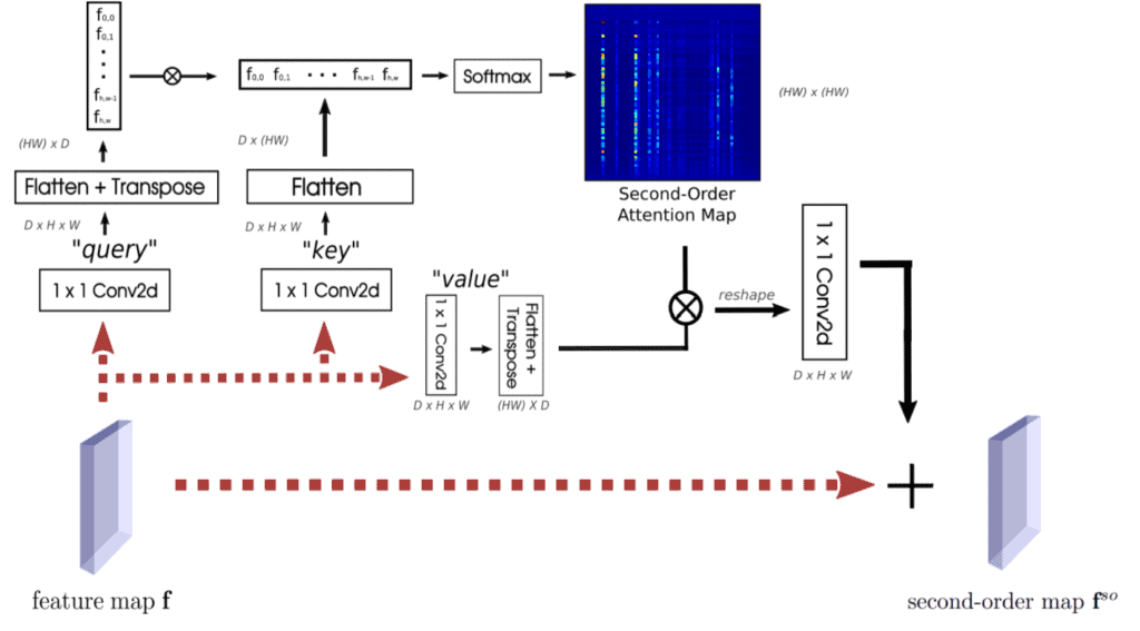
1. Remember the feature map f from earlier? We first make 3 projections of f called query q, key k and value v, all with 1×1 convolutions.
2. Each q, k and v have the exact same shape as f which is d x h x w. We first flatten all of them in the spatial dimensions to get 2D-tensors of shape d x (hw).
3. We then transpose the flattened version of q and multiply with k. Here, the matrix product q^Tk has shape hw x hw.
4. Now we take the softmax of this product z = softmax ( $\alpha $ $\cdot $ q^Tk ) along its second dimension. Some of you might have noticed, this is part where the second-order information comes into play. This effectively gives each spatial location in f  a probability distribution of all its spatial locations! In the paper, we call z the second-order attention (SOA).
5. Lastly, we multiply z with v, reshape it back to the same shape as f  (d x h x w) and pass it through another 1×1 convolution. Then we simply add it to f to get f^so.

You can think of steps 1-5 as a way to re-weight f using SOA. Since each feature in f^so now also includes information from all other features from f, the GeM pooling on f^so should also give us a global descriptor that is more robust to the challenges of image retrieval on landmark images above.

Let’s try to understand the effects of SOAs by visualising some of them on landmark images. In Figure 5, you can see when we select a spatial location with the pink star, the corresponding SOA at that location is overlaid on top of the original image. When the pink star is within landmarks, the SOA focuses on very distinctive parts of the image. When it is within background/unrelated objects, it tries to outline the silhouette of the main landmark(s) in the image. This shows that the SOAs are able to flexibly how much each feature should take in information from the other parts of the image, achieving the re-weighting goal as mentioned above. We found that utilising second-order information with SOAs help us achieve significantly better results in large-scale image retrieval datasets, and if you are interested in this field, I highly encourage you to check out our ECCV’20 paper for a more in-depth analysis.

Visualising second-order attention maps with OpenCV

In the process of doing this project, I had to constantly visualise attention maps at different locations in numerous images. I ended up having a huge pile of images and attention maps and it became impossible for me to pick out suitable examples to study with! Luckily, OpenCV allows us to interactively select a location with just a couple of mouse clicks and visualise the corresponding SOA.

Let’s take this gorgeous image of the Eiffel tower and call it “eiffel.jpg”

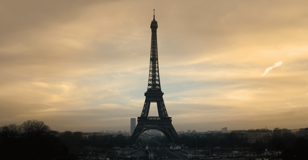
We can load up the image with OpenCV:

import cv2
image = cv2.imread("eiffel.jpg")
cv2.namedWindow("image")

# initialize the list of reference points and boolean indicating
refPt = []

Now we have to create a callback function called click_and_draw_rect() which is triggered by drawing a rectangle on the OpenCV image window:

def click_and_draw_rect(event, x, y, flags, param):
	# grab references to the global variables
	global refPt
	# if the left mouse button was clicked, record the starting
	# (x, y) coordinates	
      if event == cv2.EVENT_LBUTTONDOWN:
		refPt = [(x, y)]
	# check to see if the left mouse button was released
	elif event == cv2.EVENT_LBUTTONUP:
		# record the ending (x, y) coordinates and indicate that
		refPt.append((x, y))
		# draw a rectangle around the region of interest
		cv2.rectangle(image, refPt[0], refPt[1], (0, 255, 0), 2)
		cv2.imshow("image", image)

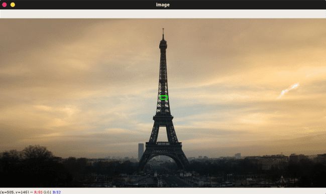
You should now see the (green) rectangle you’ve drawn on the “image” window. What has happened now is that the click_and_draw_rect() has recorded the locations of the opposing corners of the triangle and appended them to refPt.

Now, we would like to extract the SOA at this location. Let’s take a look at this function called draw_soa_map(img, model, refPt).

import torch
import torch.nn.functional as F
from torchvision import transforms
import numpy as np
import matplotlib.pyplot as plt
import matplotlib.patches as patches
from matplotlib.patches import Arrow, Circle
from mpl_toolkits.axes_grid1 import make_axes_locatable

def draw_soa_map(img, model, refPt):
    # imagenet statistics for normalization
    mean = [0.485, 0.456, 0.406]
    std  = [0.229, 0.224, 0.225]

    normalize = transforms.Normalize(mean=mean, std=std)
    transform = transforms.Compose([
            transforms.ToTensor(),
            normalize,
        ])

    img_tensor = transform(img).unsqueeze(0).cuda()

    fig = plt.figure(dpi=200)
    ax = fig.add_subplot(111)
    ax.set_xticks([])
    ax.set_yticks([])
    # h and w are the height and width of our input image
    h, w = img_tensor.shape[-2:]

    with torch.no_grad():
        ######################################################
        # Here, model (one of the function's arguments) is a torch.nn.Module class, which is our deep CNN. In this case, we are using ResNet-101
        # let's say calling model.features(img_tensor) returns two tensors, the first of which is the final feature layer f with size 2048 * h//32 * w//32
        # the second of which is the second-order attention map from the last layer with size (h//32 * w//32)**2
        #######################################################
        f, soa_last = model.features(img_tensor)
        
        # h_last and w_last are the height and width of final feature map f
        h_last, w_last = f.shape[-2:]

        # now we try to find the location of the centre of the rectangle we drew, i.e. refPt, projected onto f
        pos_h_last, pos_w_last = int(((refPt[0][1] + refPt[1][1]) / 2) // 32), int(((refPt[0][0] + refPt[1][0]) / 2) // 32)
        # and the location of the original image
        pos_h, pos_w = ((refPt[0][1] + refPt[1][1]) / 2), ((refPt[0][0] + refPt[1][0]) / 2)

        # then we retrieve the SOA at that location
        soa_last = soa_last.view(1, h_last, w_last, -1)
        self_soa_last = soa_last[:, pos_h_last, pos_w_last, ...].view(-1, h_m1, w_m1)
        self_soa_last = F.interpolate(self_soa_last.unsqueeze(1), size=(h, w), mode='bilinear').squeeze()
        # overlay the attention on the original image with alpha mask
        ax.imshow(img)
        ax.imshow(self_soa_m1.cpu().numpy(), cmap='jet', alpha=.65)
        # add a circle at the centre of the rectangle we draw to indicate where the soa is selected from
        ax.add_patch(Circle((pos_w1, pos_h1), radius=5, color='white', edgecolor='white', linewidth=5))

        plt.tight_layout()

    # redraw the canvas
    fig.canvas.draw()

    # convert canvas to image
    img_cv2 = np.fromstring(fig.canvas.tostring_rgb(), dtype=np.uint8, sep='')
    img_cv2  = img_cv2.reshape(fig.canvas.get_width_height()[::-1] + (3,))

    # img_cv2 is rgb, convert to opencv's default bgr
    img_cv2 = cv2.cvtColor(img_cv2,cv2.COLOR_RGB2BGR)
    
    return img_cv2

I know, this function is rather long and complicated! However, all it’s doing is finding what’s the correct location in the feature map f we should select. As the last feature map of most CNNs (in our case, ResNet-101) has much lower spatial resolution than the original image, we have to divide by the scale difference and round-off the location of the rectangle’s centre from the original image to the feature map’s size (in the case of ResNet-101, f  is 1/32nd the input image’s size). Remember we mentioned earlier the soa has shape hw x hw ? In the above function, we reshape it to h x w x h x w  and using pos_h_last, pos_w_last  which we calculated from our reference points, we can get the SOA at that location, which is of shape h x w. Quite easily done!

Last but not least, we call this function after the mouse callback function earlier, which is still within the while loop:

  from PIL import Image
    # if there are two reference points, then crop the region of interest
    # from the image and display it
    if len(refPt) == 2:
        # display soa
        soa = draw_soa_map(Image.open("eiffel.jpg"), model, refPt)
        cv2.imshow("Second order attention", soa)
        cv2.waitKey(20)

# close all open windows
cv2.destroyAllWindows()

(Note: model is a torch.nn.Module class of the CNN we use. For more details please see our GitHub repo.)

And you should see the SOA pop-up in a new window:

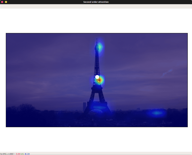
Now try drawing the rectangle within the sky on the original window.

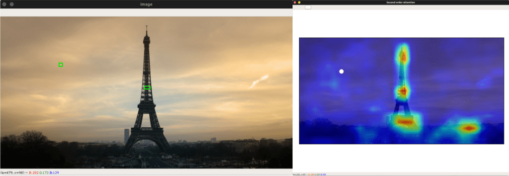
The SOA is more spread-out and silhouetting the landmarks in the image, which confirms our observation earlier!

With this functionality offered by OpenCV, I was able to create a GIF rather effortlessly, which is great for teasing your work on social media!

Conclusion

Although Deep Learning has contributed a lot  to image retrieval, state-of-the-art landmark retrieval techniques are still far from perfect. There is a constant tug-of-war between the accuracy of local aggregation methods and the efficiency of global single-pass methods. I hope my work has bridged this gap ever so slightly and we can see some truly amazing works coming in the future, which is both fast and accurate enough to work on an extremely large scale – perhaps retrieving billions of images in a blink of an eye!