
About the author:
Pau Rodríguez is a research scientist at Element AI, Montreal. He earned his Ph.D. in computer science from the Universitat Autònoma de Barcelona. His research interests include meta-learning and computer vision.
Image annotation can be a bottleneck for the applicability of machine learning when a costly expert annotation is needed. Some examples are medical imaging, astronomy, or botanics.
To alleviate this problem, few-shot classification aims to train classifiers from a small (few) number of samples (shot). A typical scenario is one-shot learning, with only one image per class. Another is zero-shot learning, where classes are given to the model in a different format. For instance, I could tell you “roses are red, the sky is blue” and you should be able to classify them without actually seeing any picture.
Recent works leverage unlabeled data to boost a few-shot performance. Some examples are label propagation and embedding propagation. These methods are in the “transductive” and “semi-supervised” learning (SSL) category. In this post, I will first overview the field of few-shot learning. Then I will explain transductive and SSL by using label propagation and embedding propagation as examples.
Few-shot Classification
In the typical few-shot scenario introduced by Vinyals et al., the model is presented with episodes composed of a support set and a query set. The support set contains information about the categories into which we want to classify the queries. For instance, the model could be given a picture of a computer and a tablet and from there it should be able to classify these two categories. In fact, models are usually given five categories (5-way), and one (one-shot) or five (five-shot) images per category. During training, the model is fed with these episodes and it has to learn to correctly guess the labels of the query set given the support set. The categories seen during training, validation, and testing, are all different. This way we know for sure that the model is learning to adapt to any data and not just memorizing information from the training set. Although most algorithms use episodes, different algorithm families differ in how to use these episodes to train the model. Next, I will introduce three families of algorithms: metric learning, gradient-based learning, and transfer learning.
Metric learning approaches
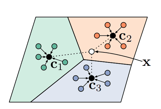
Currently, the simplest and most popular way of few-shot learning is metric learning. In this paradigm, the model learns to project images into a space where similar classes are close together given some distance metric, while different classes lay further apart. Perhaps the most well-known few-shot learning model is k-nearest neighbors, which would assign queries to the label of the closest supports. In fact, prototypical networks (Snell et al.), one of the most popular few-shot algorithms at this moment, is based on the same metric learning principle, see Figure 1.
Gradient-based approaches
Algorithms in this category, such as Model Agnostic Metalearning or MAML (Finn et al.), learn a good network initialization so that any problem can be solved by fine-tuning the model on a given support set. For each training iteration, MAML optimizes copies of the network parameters on multiple episodes at the same time and then updates the original weights by doing back-propagation through all these optimizations. MAML has inspired many posterior works such as Reptile, iMAML, or ANIL.

Transfer learning approaches
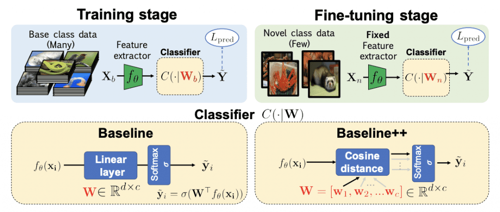
Recently, transfer learning approaches have become the new state-of-the-art for few-shot classification. Methods like Dynamic Few-Shot Visual Learning without Forgetting (Gidaris & Komodakis), pre-train a feature extractor in a first stage, and then, in a second stage, they learn to reuse this knowledge to obtain a classifier on new samples. Due to its success and simplicity, transfer learning approaches have been named “Baseline” on two recent papers (Chen et al., Dhillon et al.).
Needless to say, there are many works that are not cited here and deserve some time, as well as bayesian or generative methods. However, the purpose of this post is to introduce transductive few-shot learning, which comes next after this brief introduction to few-shot learning.
Transductive Few-shot Learning
The most common classification scenario in machine learning is the inductive one (or not so, as you will see later…). In this scenario, we have to learn a function that produces a label for any given input. Differently, in the transductive scenario, the model has access to all the unlabeled data that we want to classify, and it only needs to produce labels for those samples (as opposed to every possible input sample). In practice, transduction is used as a form of semi-supervised learning, where we have some unlabeled samples from which the model can obtain extra information about the data distribution to make better predictions. In few-shot learning, transductive algorithms make use of all the queries in an episode instead of treating them individually. One possible criticism of this scenario is that there are usually 15 queries per class, and it is unrealistic that we get balanced unlabeled data in real life applications. As Nichol et al. point in their paper, note that many few-shot algorithms are already transductive thanks to batchnorm.
Recently, transductive algorithms have increased in popularity in few-shot classification thanks to the work of Liu et al. who leverage a transductive algorithm called label propagation. So, what is label propagation?


Label Propagation
Label propagation (Zhu & Ghahramani) is an algorithm that consists in transmitting label information through the nodes of a graph, where nodes correspond to labeled and unlabeled samples. This graph is built based on some similarity metric between embeddings so nodes that are close in the graph are supposed to have similar labels. The main advantage with respect to other algorithms such as KNN is that label propagation respects the structure of the data. Here is an example I made:
Although this propagation algorithm is iterative, (Zhou et al.) proposed a closed-form solution. The algorithm is as follows:
1. Compute the similarity matrix $W$of the nodes. In this matrix $W_{i,j}$ the similarity between the node $i$ and the node $j$. The diagonal is zeroed to avoid self-propagation.
2. Then compute $S=D^{-\frac{1}{2}}WD^{-\frac{1}{2}}$ the Laplacian matrix, which can be seen as a matrix representation of the graph.
3. Get the propagator matrix $P=(I-\alpha S)^{-1}$. Basically, this matrix tells you how much label information you have to transmit from one node to another.
4. Finally, given a matrix $Y$ where each row is the one-hot encoding of a node, and most rows are made of 0s (unlabeled samples) while some contain a 1 in the corresponding class, the final labels $\hat{Y}$ are $PY$.
The matrix inverse is an expensive operation and makes it difficult to apply for large datasets, but luckily few-shot episodes are small. Thus, Liu et al. proposed a Transductive Propagation Network (TPN) for Few-shot Learning, shown in the Figure below:
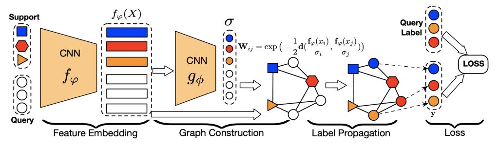
Figure 5. Transductive propagation network. Image features are extracted with a CNN. Then these features are used to build a graph with similarity matrix $W.$ In order to have 0s for non-adjacent nodes a Radial Basis Function is used. is predicted by another neural network ($g_{\Phi}$). Credit: Liu et al.
The idea is that the labels of the support set get transmitted to the query set through the graph. This architecture turned out to be very effective, obtaining state-of-the-art results and inspiring new state-of-the-art methods such as embedding propagation.
Embedding Propagation
As explained by Chapelle et al., semi-supervised learning and transductive learning algorithms make three important assumptions on the data: smoothness, cluster, and manifold assumptions. In the recent embedding propagation paper published at ECCV2020, the authors build on the first assumption to improve transductive few-shot learning. Concretely, this assumption says that points that are close in embedding space must be close also in label space (similar points have similar labels). In order to achieve this smoothness, the authors applied the label propagation algorithm to propagate image feature information instead of label information as you can see in the next Figure:
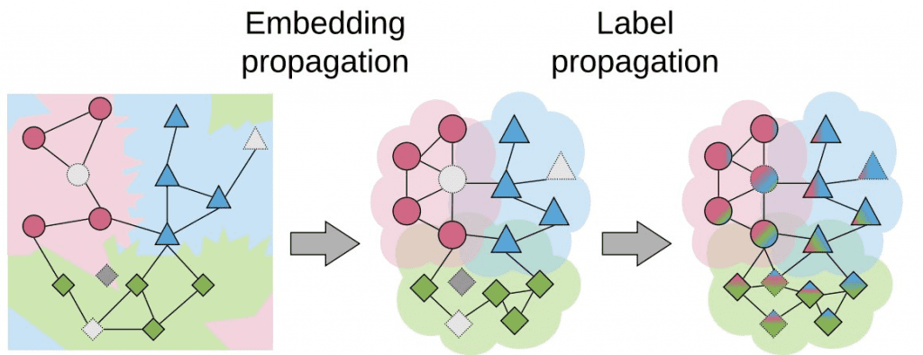
This means nodes that are similar to each other become even closer to each other, increasing the density of the embedding space. As a result, label propagation applied on these new dense embeddings achieves higher performance:

Moreover, the authors show that their method is also beneficial for semi-supervised learning and other transductive algorithms. For instance, they applied embedding propagation to the few-shot algorithm proposed by Gidaris et al. obtaining a 2% increase of performance in average. The authors provide PyTorch code in their github repository. You can use it in your model with only 3 extra lines of code:
import torch
from embedding_propagation import EmbeddingPropagation

ep = EmbeddingPropagation()
features = torch.randn(32, 32)
embeddings = ep(features)
Conclusions
Transductive learning has become a recurrent topic in few-shot classification. Here we have seen what is transductive learning and how it has improved the performance of few-shot algorithms. We have also seen some of its drawbacks, like the balance assumption of the unlabeled data. Finally, I have explained the recent embedding propagation algorithm to improve transductive few-shot classification and given some intuition on why it works.


5K+ Learners
Join Free VLM Bootcamp3 Hours of Learning