Imagine capturing the perfect landscape photo on a sunny day, only to find harsh shadows obscuring key details and distorting colors. Similarly, in computer vision projects, shadows can interfere with object detection algorithms, leading to inaccurate results. Shadows are a common nuisance in image processing, introducing uneven illumination that compromises both aesthetic quality and functional analysis.

In this blog post, we’ll tackle this challenge head-on with a practical approach to shadow correction using OpenCV. Our method leverages Multi-Scale Retinex (MSR) for illumination normalization, combined with adaptive shadow masking in LAB and HSV color spaces. This technique not only removes shadows effectively but also preserves natural colors and textures.

We’ll provide a complete Python script that includes interactive trackbars for real-time parameter tuning, making it easy to adapt to different images. Whether you’re a photographer, a developer working on augmented reality, or just curious about image enhancement, this guide will equip you with the tools to banish shadows from your images.

How Shadows Affect Image Appearance

Before diving into solutions, let’s understand shadows and their challenges in image processing. A shadow forms when an object blocks light, reducing illumination on a surface. This dims the area but doesn’t alter the object’s inherent properties.

Key points to consider,

• Shadows impact illumination, not reflectance (the object’s true color and material).
• The same object may look dark in shadow and bright in light, confusing viewers and algorithms.
• Shadows vary: soft (smooth transitions) or hard (sharp edges), needing precise detection to prevent artifacts.

Simply brightening an image won’t fix shadows; it can overexpose highlights or skew colors. Instead, effective correction separates illumination from reflectance. The image model is I = R × L, where I denotes the observed image, R denotes reflectance, and L denotes illumination. To recover R, estimate and normalize L, often using logs for stability.

Real-world examples show how shadows cause uneven lighting, which our method corrects by isolating and adjusting these components.

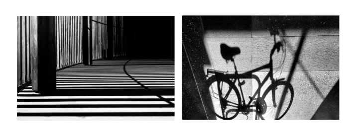
These visuals illustrate uneven lighting from shadows, guiding our approach to preserve true colors.

Understanding the Fundamentals

Before diving into the code, let’s build a solid foundation on the key concepts.

Color Spaces Explained

Images are typically represented in RGB (Red, Green, Blue), but for shadow removal, other color spaces are more suitable because they separate luminance (brightness) from chrominance (color).

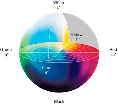
• LAB Color Space: This is a perceptually uniform color space where L represents lightness (0-100), A the green-red axis, and B the blue-yellow axis. It’s ideal for shadow correction because we can manipulate the L channel independently without affecting colors. In OpenCV, we convert using cv.cvtColor(img, cv.COLOR_BGR2LAB).

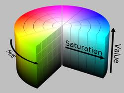
• HSV Color Space: Hue (H), Saturation (S), and Value (V). Shadows often appear as areas with low saturation and value. We use the S channel to help identify shadows, as they tend to desaturate colors.

Switching to these spaces allows us to target shadows more precisely.

Retinex Theory Basics

Retinex theory, proposed by Edwin Land in the 1970s, models how the human visual system achieves color constancy, perceiving colors consistently under varying illumination, much like how our eyes adapt to different lighting without changing perceived object colors. The core idea is that an image can be decomposed into reflectance (intrinsic object properties, like surface material) and illumination (lighting variations, such as shadows or highlights).

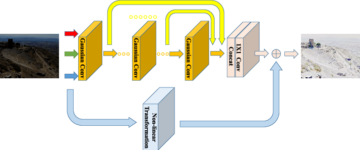
Multi-Scale Retinex (MSR) extends this by applying Gaussian blurs at multiple scales to estimate illumination, inspired by the multi-resolution processing in human vision. For each scale:

1. Blur the image to approximate the illumination component and smooth out local variations.
2. Subtract the log of the blurred image from the log of the original (to handle the multiplicative nature of illumination effects, as log transforms multiplication to addition for easier separation).
3. Average across scales for a robust estimate, balancing local and global corrections.

This results in an enhanced image with reduced shadows, improved dynamic range, and better contrast in low-light areas. In our code, we apply MSR only to the L channel for efficiency, focusing on luminance where shadows primarily affect brightness.

Shadow Detection Challenges

Simple thresholding on brightness fails because shadows vary in intensity (from subtle gradients to deep darkness) and can blend seamlessly with inherently dark objects, leading to false positives or missed areas. We need an adaptive approach that considers context:

• Combine low luminance (L < threshold) with low saturation (S < threshold), as shadows not only darken but also desaturate colors by reducing light intensity without adding new hues.
• Use morphological operations, such as closing to fill small gaps in the mask and opening to remove isolated noise specks, to refine the mask for better accuracy and continuity.
• Smooth the mask with a Gaussian blur to achieve seamless blending and prevent visible edges or halos in the corrected image.

This ensures we correct only shadowed areas without over-processing the rest of the image, maintaining natural transitions and avoiding artifacts.

Overview of the Shadow Removal Pipeline

Our pipeline processes the image step-by-step for effective shadow correction:

1. Load and Preprocess: Read the image and resize for faster preview (e.g., 50% scale).
2. Color Space Conversion: Convert to LAB (for luminance/chrominance) and HSV (for saturation).
3. Compute Retinex: Apply Multi-Scale Retinex on the L channel to create an illumination-normalized version.
4. Generate Shadow Mask: Use adaptive conditions on normalized L and S, then blur for softness.
5. Remove Shadows: Blend the original L with Retinex L in shadowed areas. For A/B channels, blend with estimated background colors to avoid color shifts.
6. Interactive Tuning: Use OpenCV trackbars to adjust strength, sensitivity, and blur in real-time.
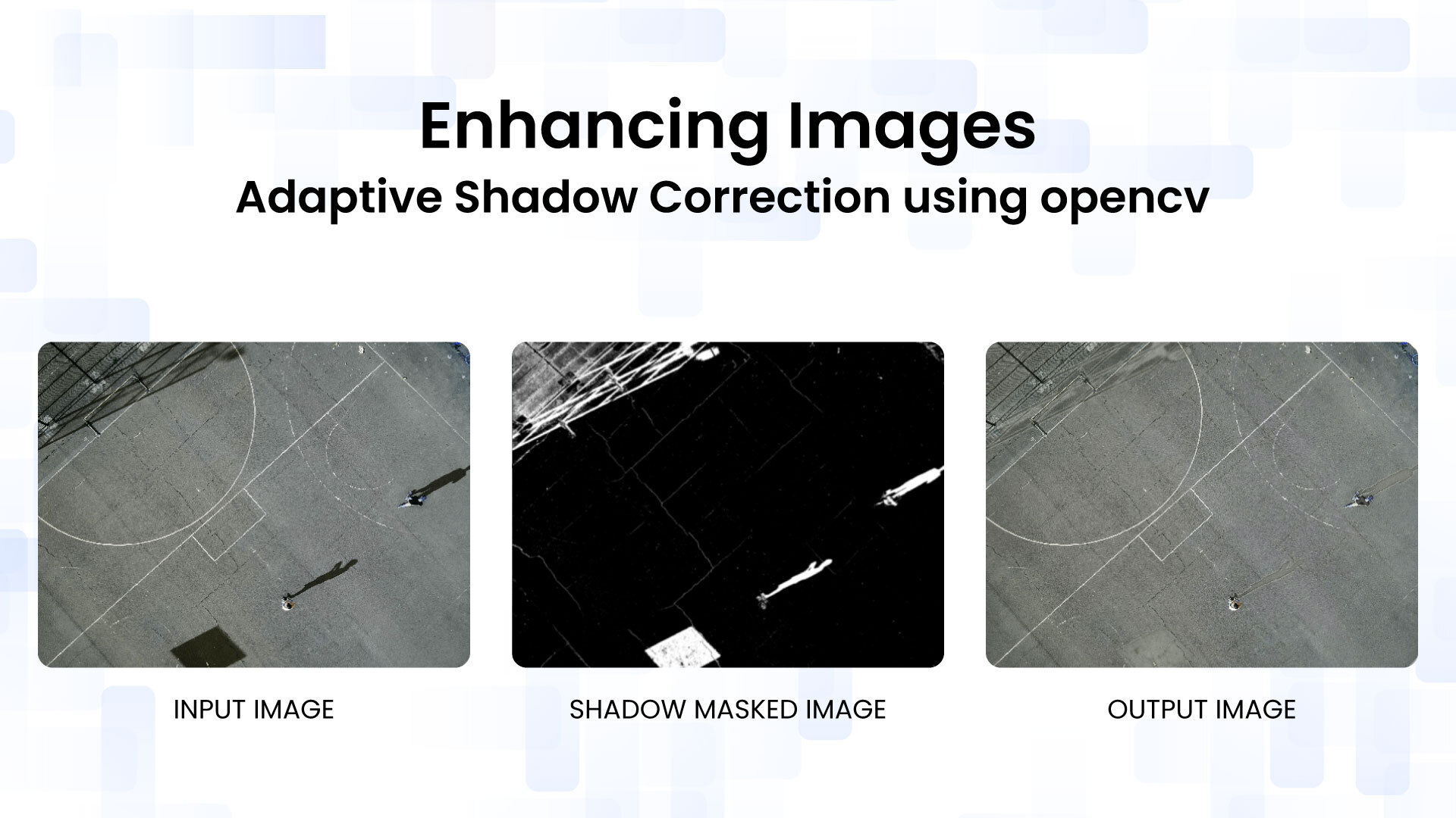
7. Display Results: Show original, mask, and corrected image side-by-side.

This approach is adaptive, meaning it responds to image content, and the parameters allow customization for various lighting conditions.

Diving into the Code: Step-by-Step Breakdown

Let’s dissect the Python script. We’ll assume you have OpenCV and NumPy installed (pip install opencv-python numpy).

Prerequisites

• Python 3.x
• OpenCV (cv2)
• NumPy (np)

Core Functions

Multi-Scale Illumination Normalization (Retinex Processing)

This function computes the Multi-Scale Retinex on the lightness channel.

def multiscale_retinex(L):
    scales = [31, 101, 301]  # Small, medium, large scales for different illumination sizes
    retinex = np.zeros_like(L, dtype=np.float32)
    for k in scales:
        blur = cv.GaussianBlur(L, (k, k), 0)  # Blur to estimate illumination
        retinex += np.log(L + 1) - np.log(blur + 1)  # Log subtraction for reflectance
    retinex /= len(scales)  # Average across scales
    retinex = cv.normalize(retinex, None, 0, 255, cv.NORM_MINMAX)  # Scale to 0-255
    return retinex

Why these scales? Smaller kernels capture fine details, larger ones handle broad shadows. The +1 avoids log(0) issues. Normalization ensures the output matches the input range.

Adaptive Shadow Detection and Mask Generation

Creates a binary shadow mask and softens it.

def compute_shadow_mask_adaptive(L, S, sensitivity=1.0, mask_blur=21):
    shadow_cond = (L < 0.5 * sensitivity) & (S < 0.5)  # Low brightness and saturation
    mask = shadow_cond.astype(np.float32)  # 0 or 1 float
    mask_blur = mask_blur if mask_blur % 2 == 1 else mask_blur + 1  # Ensure odd for Gaussian
    mask = cv.GaussianBlur(mask, (mask_blur, mask_blur), 0)  # Soften edges
    return mask

Sensitivity scales the luminance threshold, allowing tuning for faint or dark shadows. The blur prevents harsh transitions.

5K+ Learners
3 Hours of Learning

Join Free VLM Bootcamp

100K+ Learners
3 Hours of Learning

Join Free OpenCV Bootcamp

15K+ Learners
3 Hours of Learning

Join Free TensorFlow Bootcamp

10K+ Learners
8 Hours of Learning

Join Free PyTorch Bootcamp

View all AI Free Courses

Mask-Guided Shadow Removal and Color Preservation

The heart of the correction: refines the mask and blends channels.

def remove_shadows_adaptive_v3(L, A, B, L_retinex, strength=0.9, mask=None, mask_blur=31):
    kernel = cv.getStructuringElement(cv.MORPH_ELLIPSE, (7, 7))  # Elliptical kernel for morphology
    shadow_mask = cv.morphologyEx(mask, cv.MORPH_CLOSE, kernel)  # Close gaps
    shadow_mask = cv.morphologyEx(shadow_mask, cv.MORPH_OPEN, kernel)  # Remove noise
    shadow_mask = cv.dilate(shadow_mask, kernel, iterations=1)  # Expand slightly
    shadow_mask = cv.GaussianBlur(shadow_mask, (mask_blur, mask_blur), 0)  # Smooth
    mask_smooth = np.power(shadow_mask, 1.5)  # Non-linear for stronger effect in core shadows

    L_final = (1 - strength * mask_smooth) * L + (strength * mask_smooth) * L_retinex  # Blend L
    L_final = np.clip(L_final, 0, 255)  # Prevent overflow

    mask_inv = 1 - mask_smooth  # Non-shadow areas
    A_bg = np.sum(A * mask_inv) / (np.sum(mask_inv) + 1e-6)  # Average A in non-shadows
    B_bg = np.sum(B * mask_inv) / (np.sum(mask_inv) + 1e-6)  # Average B

    A_final = (1 - strength * mask_smooth) * A + (strength * mask_smooth) * A_bg  # Blend A/B
    B_final = (1 - strength * mask_smooth) * B + (strength * mask_smooth) * B_bg

    return L_final, A_final, B_final

Morphological ops refine the mask: closing fills holes, opening removes specks, dilation ensures coverage. The power function makes blending more aggressive in deep shadows. Background color estimation for A/B preserves chromaticity.

Trackbar Callback Utility

A placeholder for trackbar callbacks, as required by OpenCV.

def nothing(x):
    pass

Full Code:
The entry point handles image loading, setup, and the interactive loop.

import cv2 as cv
import numpy as np

# Retinex (compute once) 
def multiscale_retinex(L):
    scales = [31, 101, 301]
    retinex = np.zeros_like(L, dtype=np.float32)
    for k in scales:
        blur = cv.GaussianBlur(L, (k, k), 0)
        retinex += np.log(L + 1) - np.log(blur + 1)
    retinex /= len(scales)
    retinex = cv.normalize(retinex, None, 0, 255, cv.NORM_MINMAX)
    return retinex

# Adaptive Shadow Mask
def compute_shadow_mask_adaptive(L, S, sensitivity=1.0, mask_blur=21):
    shadow_cond = (L < 0.5 * sensitivity) & (S < 0.5)
    mask = shadow_cond.astype(np.float32)
    mask_blur = mask_blur if mask_blur % 2 == 1 else mask_blur + 1
    mask = cv.GaussianBlur(mask, (mask_blur, mask_blur), 0)
    return mask

#  Shadow Removal 
def remove_shadows_adaptive_v3(L, A, B, L_retinex, strength=0.9, mask=None, mask_blur=31):
    kernel = cv.getStructuringElement(cv.MORPH_ELLIPSE, (7, 7))
    shadow_mask = cv.morphologyEx(mask, cv.MORPH_CLOSE, kernel)
    shadow_mask = cv.morphologyEx(shadow_mask, cv.MORPH_OPEN, kernel)
    shadow_mask = cv.dilate(shadow_mask, kernel, iterations=1)
    shadow_mask = cv.GaussianBlur(shadow_mask, (mask_blur, mask_blur), 0)
    mask_smooth = np.power(shadow_mask, 1.5)

    L_final = (1 - strength * mask_smooth) * L + (strength * mask_smooth) * L_retinex
    L_final = np.clip(L_final, 0, 255)

    mask_inv = 1 - mask_smooth
    A_bg = np.sum(A * mask_inv) / (np.sum(mask_inv) + 1e-6)
    B_bg = np.sum(B * mask_inv) / (np.sum(mask_inv) + 1e-6)

    A_final = (1 - strength * mask_smooth) * A + (strength * mask_smooth) * A_bg
    B_final = (1 - strength * mask_smooth) * B + (strength * mask_smooth) * B_bg

    return L_final, A_final, B_final

def nothing(x):
    pass

#  Main 
if __name__ == "__main__":
    img = cv.imread("image.jpg")
    if img is None:
        raise IOError("Image not found")

    scale = 0.5
    img_preview = cv.resize(img, None, fx=scale, fy=scale, interpolation=cv.INTER_AREA)

    lab = cv.cvtColor(img_preview, cv.COLOR_BGR2LAB).astype(np.float32)
    L, A, B = cv.split(lab)
    L_retinex = multiscale_retinex(L)

    hsv = cv.cvtColor(img_preview, cv.COLOR_BGR2HSV).astype(np.float32)
    S = hsv[:, :, 1] / 255.0

    cv.namedWindow("Shadow Removal", cv.WINDOW_NORMAL)
    cv.createTrackbar("Strength", "Shadow Removal", 90, 200, nothing)
    cv.createTrackbar("Sensitivity", "Shadow Removal", 90, 200, nothing)
    cv.createTrackbar("MaskBlur", "Shadow Removal", 31, 101, nothing)

    while True:
        strength = cv.getTrackbarPos("Strength", "Shadow Removal") / 100.0
        sensitivity = cv.getTrackbarPos("Sensitivity", "Shadow Removal") / 100.0
        mask_blur = cv.getTrackbarPos("MaskBlur", "Shadow Removal")
        mask_blur = max(3, mask_blur)
        mask_blur = mask_blur if mask_blur % 2 == 1 else mask_blur + 1

        mask = compute_shadow_mask_adaptive(L / 255.0, S, sensitivity, mask_blur)

        L_final, A_final, B_final = remove_shadows_adaptive_v3(
            L, A, B, L_retinex, strength, mask, mask_blur
        )

        lab_out = cv.merge([L_final, A_final, B_final]).astype(np.uint8)
        result = cv.cvtColor(lab_out, cv.COLOR_LAB2BGR)

        #  BUILD RGB VIEW 
        orig_rgb = cv.cvtColor(img_preview, cv.COLOR_BGR2RGB)
        mask_rgb = cv.cvtColor((mask * 255).astype(np.uint8), cv.COLOR_GRAY2RGB)
        result_rgb = cv.cvtColor(result, cv.COLOR_BGR2RGB)

        combined_rgb = np.hstack([orig_rgb, mask_rgb, result_rgb])

        # Convert back so OpenCV shows correct colors
        combined_bgr = cv.cvtColor(combined_rgb, cv.COLOR_RGB2BGR)

        cv.imshow("Shadow Removal", combined_bgr)

        key = cv.waitKey(30) & 0xFF
        if key == 27 or cv.getWindowProperty("Shadow Removal", cv.WND_PROP_VISIBLE) < 1:
            break

    cv.destroyAllWindows()

Key points:

• Resizing speeds up processing for previews.
• Retinex is computed once outside the loop for efficiency.
• The loop updates on trackbar changes, recomputing the mask and correction.
• Display stacks original, mask (grayscale as RGB), and result for comparison.

Running the Code and Tuning Parameters

Setup Instructions

1. Save the code as a .py format.
2. Replace “image.jpg” with your image path (JPEG, PNG, etc.).
3. Run: python shadow_removal.py.

A window will appear with trackbars and a side-by-side view.

Output:

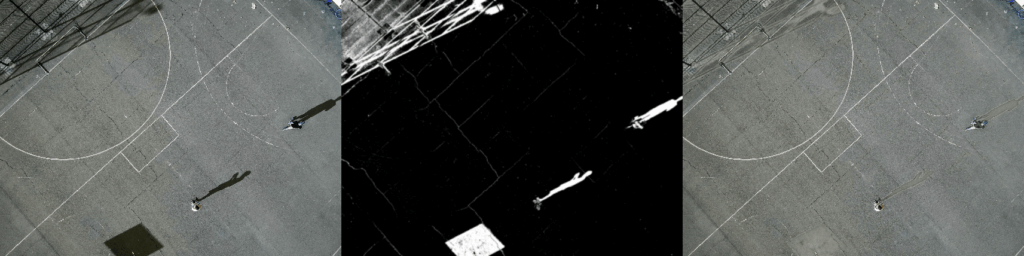
Interactive Demo

• Strength (0-2.0): Controls blending intensity. Higher values apply more correction but increase the risk of artifacts.
• Sensitivity (0-2.0): Adjusts shadow detection threshold. Lower for detecting subtle shadows, higher for aggressive ones.
• MaskBlur (3-101, odd): Softens mask edges. Larger values for smoother transitions in large shadows.

For outdoor scenes with cast shadows, increase sensitivity. For indoor low-light, reduce the strength to avoid over-brightening.

Potential Improvements and Limitations

Enhancements

• Batch Processing: Extend the pipeline to process multiple images or video frames, enabling use in real-time or large-scale applications.
• ML Integration: Incorporate deep learning models (such as U-Net) to generate more accurate, semantic shadow masks using datasets like ISTD.
• Colored Shadow Handling: Improve robustness by detecting and correcting color shifts caused by colored or indirect lighting.
• Performance Optimization: Speed up processing for large images by parallelizing Retinex scales or working on downsampled inputs.

Limitations

• Visual Artifacts: In textured regions or near shadow boundaries, blending can introduce halos or inconsistencies, requiring more refined masks.
• Computational Cost: Multi-Scale Retinex with large kernels can be slow on high-resolution images; preprocessing steps like downsampling are often necessary.
• Lighting Assumptions: The method works best for neutral (achromatic) shadows and may struggle under colored or complex illumination conditions.
• Low-Light Noise Amplification: Shadow enhancement can amplify image noise in dark areas; denoising may be needed beforehand.
• Compared to Deep Learning: OpenCV methods don’t match deep learning for complex shadow removal, and images with heavy shadowing can be tough to fully correct.

Overall, this is a solid baseline for many scenarios, and performance can be improved by tuning parameters to the specific image and lighting conditions.

Conclusion

Shadows pose a challenge in image enhancement because they affect illumination without changing object properties. This blog presented an adaptive shadow-correction pipeline using OpenCV that combines Multi-Scale Retinex with color-space–based shadow detection to reduce shadows while preserving natural colors. Interactive parameter tuning makes the method flexible across different images. Although it cannot fully match deep learning approaches for complex scenes, it provides a lightweight and effective baseline that can be further improved or extended.

Reference

Image Shadow Removal Method Based on LAB Space

Shadow Detection and Removal

Image Shadow Remover

Frequently Asked Questions