Object detection methods published recently have pushed the state of the art (SOTA) on a popular benchmark  – MS COCO dataset. Let’s take a closer look at these methods.

But first, we will start with an introduction.

Object Detection: Previous Methods

There are mainly two types of state-of-the-art object detectors.

On the one hand, we have two-stage detectors, such as Faster R-CNN (Region-based Convolutional Neural Networks) or Mask R-CNN. These use a Region Proposal Network (RPN) to generate regions of interest in the first stage and send the region proposals down the pipeline for object classification and bounding-box regression. Such models reach the highest accuracy rates, but are typically slow. 

On the other hand, we have single-stage detectors, such as YOLO (You Only Look Once) and SSD (Single Shot MultiBox Detector). They treat object detection as a simple regression problem by taking an input image and learning the class probabilities and bounding box coordinates (Figure 1). Such models reach lower accuracy rates, but are much faster than two-stage object detectors. One of the main components of these models is the use of generated priors (or anchors) which are boxes of various sizes and aspect ratios that serve as detection candidates.

CornerNet: Detecting Objects as Paired Keypoints

With the knowledge of that background, now we are ready to discuss CornerNet.

What is so special about it?

First, it eliminates the use of anchor boxes, which were popular in previous single-stage methods. CornerNet represents a bounding box as a pair of keypoints, the top-left corner and the bottom-right corner.

Second, the method introduces a new type of pooling layer – corner pooling  –  that helps the network better localize corners.

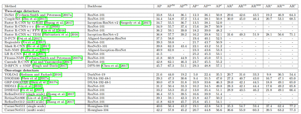
Last, but not least, the performance! Corner-Net achieves 42.2% AP on MS COCO, which is, as the authors claim, the best result compared to all existing by that time one-stage detectors.

Sounds exciting? Let’s dive into the details.

Overview

As we can see from Figure 2, CornerNet uses hourglass network as the backbone, followed by two prediction modules. One module is for the top-left corners, while the other one is for the bottom-right corners. Each module consists of its own corner pooling module (which we will discuss later) to pool features from the hourglass network before predicting the heatmaps, embeddings, and offsets.

Both predicted sets of heatmaps have c channels, where c is the number of categories, and is of size HW. There is no background channel. Each channel is a binary mask indicating the locations of the corners for a class.

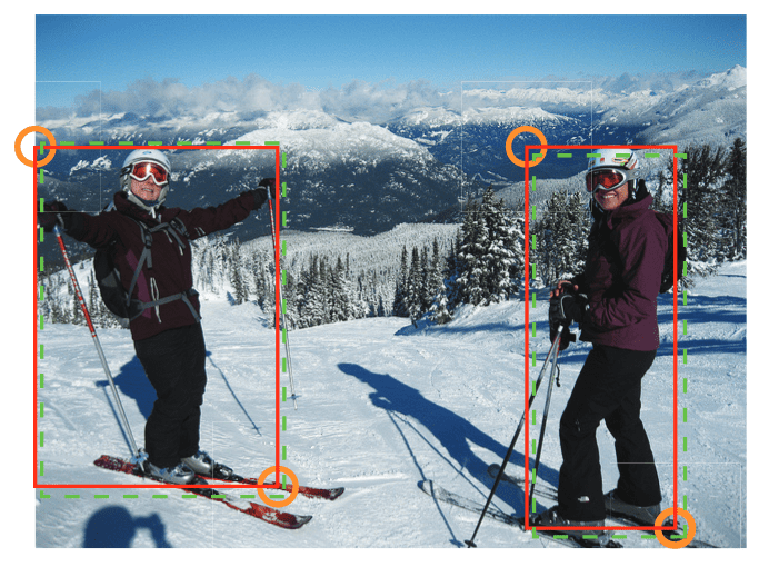
Additionally, for each detected corner the network predicts an embedding vector such that the distance between the embeddings of two corners from the same object is small (Figure 3). An object bounding box is generated if the distance is less than a threshold. The bounding box is assigned a confidence score, which is equal to the average score of the corner pair.

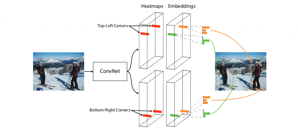
To produce tighter bounding boxes, the network also predicts offsets to slightly adjust the locations of the corners. After that, a simple post-processing algorithm including NMS (Non-maximum Suppression) is used to generate bounding boxes from the heatmaps, embeddings, and offsets.

Corner Detection

For each corner, there is one ground-truth positive location, and all other locations are negative. During training, instead of equally penalizing all negative locations, the authors reduce the penalty given to the negative locations within some radius around the positive location. This is because a pair of false corners, when close to their respective ground truth locations, can still produce a box that sufficiently overlaps the ground-truth box (Figure 4).

Corner Pooling Module

So, how are the corners detected?

As it was mentioned above, for this case a new type of pooling layer called “Corner pooling” is proposed, whose function is to help the network localize corners.

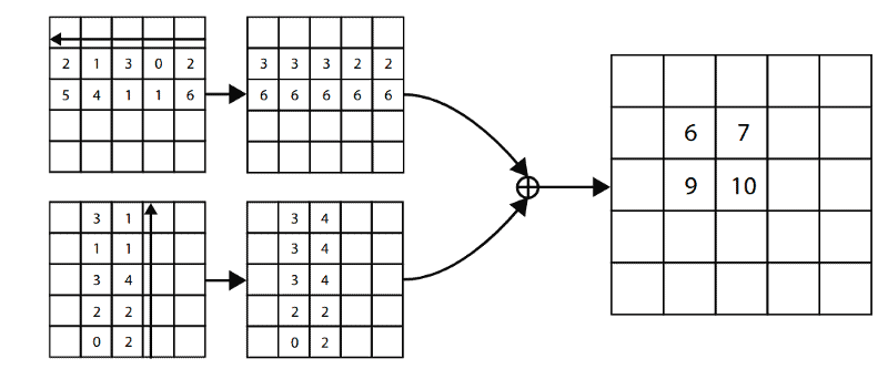
To better understand how it works, let’s have a look at Figure 5.

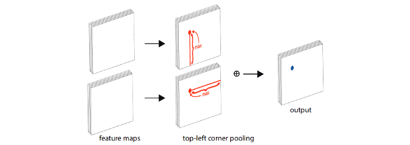
The layer detects the boundary feature of the same object in a row and a column, hence the intersection of this row and the column is the corner. Technically, this new pooling layer is a sum of two forwarded pooling layers, where the directions depend on which corner it is calculating for (from right to left and bottom-up for top-left corner pooling as in Figure 6, bottom-right corner is calculated opposite to its direction).

Prediction Module

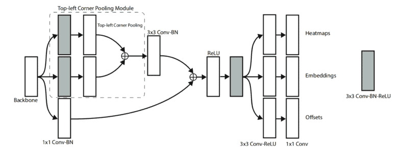
The architecture of the prediction module is shown in Figure 7.

The first part of the module is a modified version of the residual block: it first processes the features from the backbone using two 3×3 convolution modules and then applies a top-left corner pooling layer. The pooled features are then fed into a 3×3 Conv-BN layer and added back to the projection shortcut. The modified residual block is followed by a convolutional block and then is split into 3 separate branches to produce the heatmaps, embeddings, and offsets.

Training Details

• No pretraining is performed, weights are randomly initialized.
• The input resolution of the network is 511×511 and the output heatmap size is 128×128.
• Data augmentation includes random horizontal flipping, random scaling, random cropping and random color jittering, which includes adjusting the brightness, saturation and contrast of an image.
• Adam is used to optimize the training loss:

To be specific, let’s give a little bit more information about each term in the equation above:

L_det is the detection loss, which is responsible for proper corner detection and is a variant of focal loss;

L_pull is the grouping loss, used to pull corners of one object together;

L_push, is, on the opposite, used to separate corners of different objects;

L_off is the smooth L1 loss used for offset correction;

and α, β and γ are parameters, which are set to 0.1, 0.1 and 1 respectively.

Test Details

• Both the original and flipped images are used.
• The original resolution of the image is maintained and is padded with zeros before feeding it to CornerNet.
• Soft-nms method is applied to the detections and only the top 100 of them are reported.
• The average inference time is 244ms per image on a Titan X (PASCAL) GPU.

Results

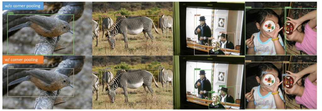
Let’s proceed to the results. You can find some examples in favor of using corner pooling on Figure 8. And comparison of CornerNet with other methods are shown on Figure 9. Note that the results are provided for two types of evaluation: single-scale and multi-scale. With the latter, CornerNet achieves an AP of 42.2% on the MS COCO dataset.

CornerNet Code

Bonus for those who made it till the end – link to the code, generously provided by the authors: 

https://github.com/princeton-vl/CornerNet.