Modern Computer Vision (CV) and Video Analytics (VA) problems are solved with a combination of traditional methods and Deep Learning (DL). Deep Neural Network Inference becomes a crucial tool in the domain, but integrating it into the application and the further deployment is sometimes non-trivial — especially if the algorithm is built with multiple DL networks. Moreover, today’s hardware platforms are heterogeneous and may run different portions of the application in parallel. Managing a complex workload on such a platform effectively becomes a problem — and here comes OpenCV G-API! This article gives a brief overview of the module, how it can be used to express complex modern CV/DL algorithms, and how to get performance out of it.

The problem of pipelining

Before we dive deep into details of G-API programming in C++, let’s review what a regular video analytics application looks like in the year 2020. Modern complex CV workloads are usually compute-hungry. A typical CV application combines decode, DL inference, image pre- and post-processing, and some custom application code or domain logic — and to illustrate this, we will build a very basic “privacy masking” application with OpenCV, G-API, and OpenVINO™ Inference Engine.

Example: Privacy Masking Pipeline

The idea of the application is simple: having a video stream, to identify and protect regions containing sensitive information — in our case, let it be faces and vehicle license plates. Example of the running application is shown in Figure 1.

Schematically the application data flow can be represented as a graph as shown in Figure 2.

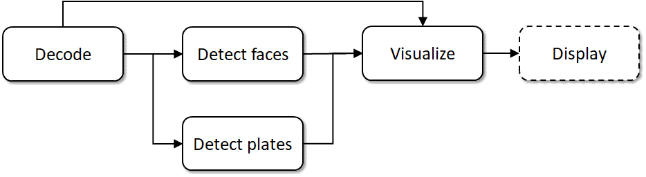
This graph consists of the following nodes, or steps:

• Reading and decoding a video stream, done via cv::VideoCapture;
• Object detection with two SSD-based networks, scored by Inference Engine;
• Custom SSD network output processing and visualization code;
• Displaying results in the user interface.

Further in the article we will refer to these steps as to “DEC”, “FD”, “PD”, “VIS”, and “DISP” appropriately.

In our example, we will use the following DL models available in OpenVINO™ Open Model Zoo:

• vehicle-license-plate-detection-barrier-0106
• face-detection-retail-0005

Note that the first network detects objects of two kinds — vehicles and license plates. In our sample, we need to process license plates only so we will implement a custom processing (filtering) for this detector.

Naive execution

If we implement this application the way we think of it, we get a naïve execution sequence for every video frame we process, like in Figure 3:

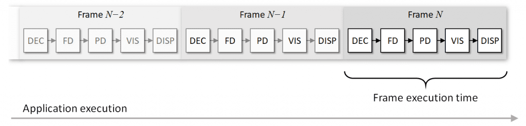
Here steps are executed sequentially, every video frame takes time ~t to process, and every new output image arrives in time ~t. Duration t may slightly change from frame to frame since the number of detected objects may vary.

Pipelined execution

Obviously, the above execution flow is far from ideal. Today’s compute platforms are usually heterogeneous and may have different blocks on-board which are able to run in parallel. For example, there may be:

• a multi-core CPU;
• a GPU, integrated or discrete;
• special HW blocks on the SoC, e.g. for media decoding or image signal processing (ISP);
• extra accelerators connected via PCIe or USB (e.g.: Altera® FPGA card or Intel® Movidius™ Neural Compute Stick).

In this case, maximizing the overall application performance entails fully loading all parallel compute blocks at the same time. This technique is called “pipelining”; an example of the execution flow with the technique applied is shown in Figure 4.

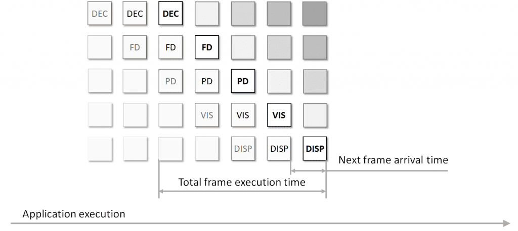
Though the frame processing latency may not really change, every new processed result arrives to the consumer faster than in the serial mode — resulting in a higher overall throughput. This assumes, however, that every block can really run in parallel and every block executes in nearly the same amount of time. In reality it rarely happens — since the system may be loaded with something else, different stages of the pipeline may take significantly different time, and some stages running in parallel may affect each other’s performance.

Pipelining challenges

Utilizing a pipelining technique looks reasonable for video stream processing with CV and DL, but how can we get it working? There is always a way to do pipelining manually and manage threads, synchronization, and data flow on our own. However, implementing this approach requires extra knowledge, is still error-prone, and does not scale well. What if the algorithm changes, e.g. we add a new stage to our pipeline? What if we move to another platform with different options available for offload? For example, offloading inference to an external accelerator may require managing multiple asynchronous inference requests at a time. With the manual approach, we need to change things manually as well — and probably repeat the whole debugging cycle.

A technological approach to the problem is to utilize computer machinery and automate the way code is pipelined. If we do any changes in the algorithm or run it on a machine with a different configuration, a framework can reason automatically how to adjust the pipeline execution after these changes.

Existing solutions

There are existing frameworks available to address the pipelining problem, with their pros and cons — ranging from a lower-level Intel® Threading Building Blocks library to higher-level frameworks like GStreamer. The Khronos® Group also defines a pipelining extension to the OpenVX™ standard for graph-based computer vision to address exactly the same problem.Now, since version 4.2, OpenCV has got its own thing — OpenCV G-API has been extended to support DL inference and video stream processing. The rest of this article explains the core principles of G-API and illustrates how workloads like this one map to this new framework.

Brief introduction to G-API

G-API (stands for “Graph API”) is not a new OpenCV module — it was first introduced in the most recent major OpenCV 4.0 release back in the year 2018. G-API is positioned as a next level optimization enabler for computer vision, focusing not on particular CV functions but on the whole algorithm optimization; more on this in these slides.

The idea behind G-API is that if an algorithm can be expressed in a special embedded language (currently in C++), the framework can catch its sense and apply a number of optimizations to the whole thing automatically. Particular optimizations are selected based on which kernels and backends are involved in the graph compilation process, for example, the graph can be offloaded to GPU via the OpenCL backend, or optimized for memory consumption with the Fluid backend. Kernels, backends, and their settings are parameters to the graph compilation, so the graph itself does not depend on any platform-specific details and can be ported easily.

Programming model explained

Building graphs is easy with G-API. In fact, there is no notion of graphs exposed in the API, so the user doesn’t need to operate in terms of “nodes” and “edges” — instead, graphs are constructed implicitly via expressions in a “functional” way. Expression-based graphs are built using two major concepts: operations and data objects.

In G-API, every graph begins and ends with data objects; data objects are passed to operations which produce (“return”) their results — new data objects, which are then passed to other operations, and so on. Programmers can declare their own operations, G-API does not distinguish user-defined operations from its own predefined ones in any way.

After the graph is defined, it needs to be compiled for execution. During the compilation, G-API figures out what the graph looks like, which kernels are available to run the operations in the graph, how to manage heterogeneity and to optimize the execution path. The result of graph compilation is a so-called “compiled” object. This object encapsulates the execution sequence for the graph inside and operates on real image data. Programmers can set up the compilation process using various compilation arguments. Backends expose some of their options as these arguments; also, actual kernels and DL network settings are passed into the framework this way.

G-API supports graph compilation for two execution modes, regular and streaming, producing different types of compiled objects as the result.

• Regular compiled objects are represented with class GCompiled, which follows functor-like semantics and has an overloaded operator(). When called for execution on the given input data, the GCompiled functor blocks the current thread and processes the data immediately — like a regular C++ function. By default, G-API tries to optimize the execution time for latency in this compilation mode.
• Starting with OpenCV 4.2, G-API can also produce GStreamingCompiled objects that better fit the asynchronous pipelined execution model. This compilation mode is called “streaming mode”, and G-API tries to optimize the overall throughput by implementing the pipelining technique as described above. We will use both in our example.

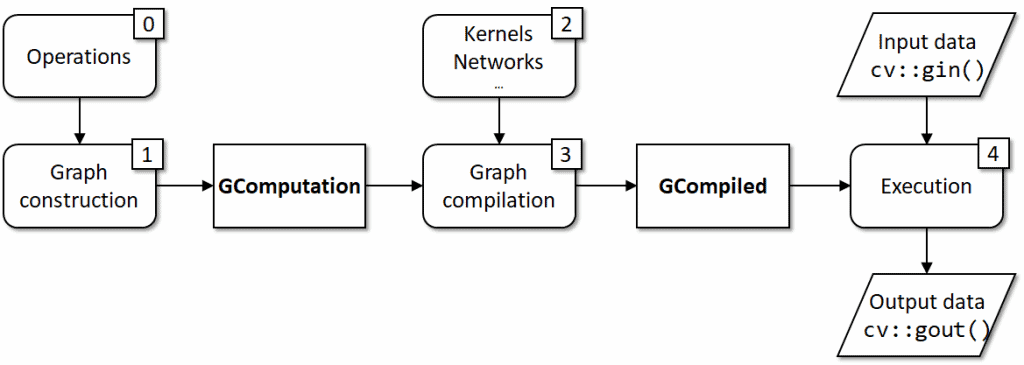
The overall process for the regular case is summarized in Figure 5. The graph is built with operations so having operations defined (0) is a basic prerequisite; a constructed expression graph (1) forms a cv::GComputation object; kernels (2) which implement operations are the basic requirement to the graph compilation (3); the actual execution (4) is handled by a cv::GCompiled object with takes input and produces output data.

Development workflow explained

One of the ways to organize a G-API development workflow is presented in Figure 6.

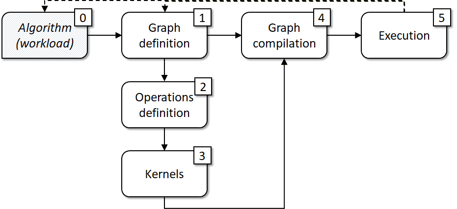
Basically, it is a derivative from the programming model illustrated in the previous chapter (Figure 5). We start with an algorithm or a data flow in mind (0), mapping it to a graph model (1), then identifying what operations we need (2) to construct this graph. These operations may already exist in G-API or be missing, in the latter case we implement the missing ones as kernels (3). Then we decide which execution model fits our case better, pass kernels and DL networks as arguments to the compilation process (4), and finally switch to the execution (5). The process is iterative, so if we want to change anything based on the execution results, we get back to steps (0) or (1) (a dashed line).

In the next section we will apply this simple process to implement our sample with G-API.

Implementing the privacy masking pipeline with G-API

Based on the described process, the workload implementation consists of three steps:

• Mapping our workload to the graph structure;
• Identifying and implementing the missing parts;
• Configuring and running the pipeline.

This section covers every step in detail.

Mapping the workload to G-API

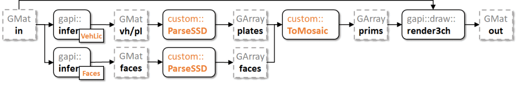
It’s time to map our original example (Figure 2) to G-API. We will use OpenCV’s cv::VideoCapture to access the video stream; G-API already comes with inference and rendering APIs, the missing parts in our workload are functions that parse detection output and convert it to G-API’s Mosaic primitives (highlighted with orange in Figure 7).

Declaring networks

In G-API, inference is a generic (template) operation and particular networks are defined with a special macro G_API_NET:

G_API_NET(VehLicDetector, <cv::GMat(cv::GMat)>, "vehicle-license-plate-detector");
G_API_NET(FaceDetector,   <cv::GMat(cv::GMat)>,                  "face-detector");

G-API tries to be type-safe so operations and networks are actually C++ types. Here we declare two types — “VehLicDetector” and “FaceDetector”, and their calling conventions — both take a cv::GMat input and produce a cv::GMat output. Third argument to each macro is a string identifier, which is used by G-API internally; the identifiers need to be unique in the scope of a single graph.

Declaring kernels

Next, we need to parse detections from the SSD format to arrays of rectangles. This operation is generally referred to as “post-processing”, so here is ours:

using GDetections = cv::GArray<cv::Rect>;

G_API_OP(ParseSSD, <GDetections(cv::GMat, cv::GMat, int)>, "custom.privacy_masking.postproc") {
    static cv::GArrayDesc outMeta(const cv::GMatDesc &, const cv::GMatDesc &, int) {
        return cv::empty_array_desc();
    }
};

Our post-processing operation takes three parameters — the SSD result blob, the original input image, and an integer class to filter objects out (remember our first detector from OpenVINO™ Open Model Zoo detects both vehicles and license plates).

Finally, we need an operation to convert our detection data to G-API rendering primitives:

using GPrims = cv::GArray<cv::gapi::wip::draw::Prim>;

G_API_OP(ToMosaic, <GPrims(GDetections, GDetections)>, "custom.privacy_masking.to_mosaic") {
    static cv::GArrayDesc outMeta(const cv::GArrayDesc &, const cv::GArrayDesc &) {
        return cv::empty_array_desc();
    }
};

Note that in OpenCV 4.4 the rendering functionality is declared under “wip” namespace. It means that it is already functional but is still experimental so the API may change in the future versions.

Constructing the pipeline

Now when we have all our extra operations defined, it’s time to construct the graph itself. Here it is:

cv::GMat in;
cv::GMat blob_plates = cv::gapi::infer<custom::VehLicDetector>(in);
cv::GMat blob_faces  = cv::gapi::infer<custom::FaceDetector>(in);

// VehLicDetector from Open Model Zoo marks vehicles with label "1" and
// license plates with label "2", filter out license plates only.
cv::GArray<cv::Rect> rc_plates = custom::ParseSSD::on(blob_plates, in, 2);

// Face detector produces faces only so there's no need to filter by label,
// pass "-1".
cv::GArray<cv::Rect> rc_faces  = custom::ParseSSD::on(blob_faces, in, -1);

cv::GMat out = cv::gapi::wip::draw::render3ch(in, custom::ToMosaic::on(rc_plates, rc_faces));

cv::GComputation graph(in, out);

Our graph starts with declaring an “empty” data object “in”. Note that in fact G-API data objects are not associated with any data but only express that there is some data — and these objects are used just to connect the operations. The real data gets into the pipeline only when it is compiled and is ready for execution.

We use “VehLicDetector” and “FaceDetector” types as template arguments to generic function “cv::gapi::infer<>()”. Since both networks are defined with a single input, these specializations of “infer” require only a single argument as well.

The produced detections are passed to our first custom operation “ParseSSD”. Every operation type we declare with G_API_OP has a static method “::on()” which “triggers” the operation in the graph. This method is auto-generated from the operation signature with some C++ templates magic, and again strictly follows the operation type. In fact, by calling “T::on()” we apply the operation “T” to input objects and produce new output.

Finally, we convert our detections to a list of drawing primitives with another custom operation, “ToMosaic”, and pass it to the standard “render3ch” operation as input. Here we trigger two operations in a single line.

The resulting graph is captured as an object “graph”. We specify “in” and “out” data objects as start/end markers in the special cv::GComputation constructor overload, and G-API tracks which operations were called on “in” to produce “out”, building the appropriate graph on the fly. If there is no way to trace “out” from “in”, or “out” requires more input objects than we passed (e.g. when a graph in fact has two inputs but we specified only a single one), G-API throws an exception.

Implementing kernels

Below is the OpenCV-based implementation of the “ParseSSD” operation. G-API OpenCV kernels are declared using a special macro GAPI_OCV_KERNEL. The first argument to this macro is a new type name for the kernel declared, and the second one is the type name of the operation we implement. This reads as “OCVParseSSD kernel implements ParseSSD operation”, like in traditional object-oriented programming.

GAPI_OCV_KERNEL(OCVParseSSD, ParseSSD) {
    static void run(const cv::Mat &in_ssd_result,
                    const cv::Mat &in_frame,
                    const int      filter_label,
                    std::vector<cv::Rect> &out_objects) {
        const auto &in_ssd_dims = in_ssd_result.size;
        CV_Assert(in_ssd_dims.dims() == 4u);

        const int MAX_PROPOSALS = in_ssd_dims[2];
        const int OBJECT_SIZE   = in_ssd_dims[3];
        CV_Assert(OBJECT_SIZE  == 7); // fixed SSD object size

        const cv::Size upscale = in_frame.size();
        const cv::Rect surface({0,0}, upscale);

        out_objects.clear();

        const float *data = in_ssd_result.ptr<float>();
        for (int i = 0; i < MAX_PROPOSALS; i++) {
            const float image_id   = data[i * OBJECT_SIZE + 0];
            const float label      = data[i * OBJECT_SIZE + 1];
            const float confidence = data[i * OBJECT_SIZE + 2];
            const float rc_left    = data[i * OBJECT_SIZE + 3];
            const float rc_top     = data[i * OBJECT_SIZE + 4];
            const float rc_right   = data[i * OBJECT_SIZE + 5];
            const float rc_bottom  = data[i * OBJECT_SIZE + 6];

            if (image_id < 0.f) {
                break;    // marks end-of-detections
            }
            if (confidence < 0.5f) {
                continue; // skip objects with low confidence
            }
            if (filter_label != -1 && static_cast<int>(label) != filter_label) {
                continue; // filter out object classes if filter is specified
            }

            cv::Rect rc;  // map relative coordinates to the original image scale
            rc.x      = static_cast<int>(rc_left   * upscale.width);
            rc.y      = static_cast<int>(rc_top    * upscale.height);
            rc.width  = static_cast<int>(rc_right  * upscale.width)  - rc.x;
            rc.height = static_cast<int>(rc_bottom * upscale.height) - rc.y;
            out_objects.emplace_back(rc & surface);
        }
    }
};

The “ToMosaic” operation is implemented in a similar way — here we just take an array of rectangles and turn it into an array of Mosaic drawing primitives, aligning every region geometry to the mosaic block size:

GAPI_OCV_KERNEL(OCVToMosaic, ToMosaic) {
    static void run(const std::vector<cv::Rect> &in_plate_rcs,
                    const std::vector<cv::Rect> &in_face_rcs,
                          std::vector<cv::gapi::wip::draw::Prim> &out_prims) {
        out_prims.clear();
        const auto cvt = [](cv::Rect rc) {
            // Align the mosaic region to mosaic block size
            const int BLOCK_SIZE = 24;
            const int dw = BLOCK_SIZE - (rc.width  % BLOCK_SIZE);
            const int dh = BLOCK_SIZE - (rc.height % BLOCK_SIZE);
            rc.width  += dw;
            rc.height += dh;
            rc.x      -= dw / 2;
            rc.y      -= dh / 2;
            return cv::gapi::wip::draw::Mosaic{rc, BLOCK_SIZE, 0};
        };
        for (auto &&rc : in_plate_rcs) { out_prims.emplace_back(cvt(rc)); }
        for (auto &&rc : in_face_rcs)  { out_prims.emplace_back(cvt(rc)); }
    }
};

Configuring the pipeline

Once the missing parts are done, we can finally compile and execute our graph. All we need to do now is to pack our compilation parameters and pass it to G-API.

const auto plate_model_path = cmd.get<std::string>("platm");
auto plate_net = cv::gapi::ie::Params<custom::VehLicDetector> {
    plate_model_path,                // path to topology IR
    weights_path(plate_model_path),  // path to weights
    cmd.get<std::string>("platd"),   // device specifier
};
const auto face_model_path = cmd.get<std::string>("facem");
auto face_net = cv::gapi::ie::Params<custom::FaceDetector> {
    face_model_path,                 // path to topology IR
    weights_path(face_model_path),   // path to weights
    cmd.get<std::string>("faced"),   // device specifier
};
auto kernels = cv::gapi::kernels< custom::OCVParseSSD
                                , custom::OCVToMosaic>();
auto networks = cv::gapi::networks(plate_net, face_net);

Note that this is the only place where we actually refer to  OpenVINO™ Inference Engine. G-API comes with an Inference Engine-based backend for inference, which is configured with a generic structure cv::gapi::ie::Params<>. This structure is specialized to every network type we use to form a parameters structure for the associated network. Some networks require a bit more configuration, e.g. when a network produces multiple outputs, here we can map (by name) which output layer stands for which output in the network’s return value tuple. Again, this API is type-safe and is based on the network’s type signature, as defined in G_API_NET.

Execution and results

In this section we run our workload in two different modes — traditional and streaming — and measure how it performs in each of those.

Baseline: serial mode

In “serial” mode G-API produces the graph result synchronously, when a GCompiled object is called for execution. We compile the graph with a regular compile() method, read the video manually, and implement the read/process/display loop manually as well:

cv::Mat in_frame;
cv::VideoCapture cap(input);
cap >> in_frame;

auto exec = graph.compile(cv::descr_of(in_frame),
                          cv::compile_args(kernels, networks));
do {
    exec(in_frame, out_frame);
    if (!no_show) {
        cv::imshow("Out", out_frame);
        cv::waitKey(1);
    }
} while (cap.read(in_frame));

Streaming mode

The streaming execution mode implements a pipelined execution model in G-API. The semantics of the streaming mode is different but in fact is much simpler. All we need to do is to compile the graph with compileStreaming() instead of the regular compile(), and then specify the input source to the resulting pipeline. Finally, we start the pipeline and fetch/display the results in the loop until the stream ends:

auto pipeline = graph.compileStreaming(cv::compile_args(kernels, networks));
pipeline.setSource(cv::gapi::wip::make_src<cv::gapi::wip::GCaptureSource>(input));
pipeline.start();

while (pipeline.pull(cv::gout(out_frame))) {
    if (!no_show) {
        cv::imshow("Out", out_frame);
        cv::waitKey(1);
    }
}

Full sample source code is available at the OpenCV Github repository.

Performance comparison

The sample’s resulting performance depends on many options:

• Which devices are used for inference and what the inference precision per each network is (CPU/INT8, CPU/FP32, GPU/FP16);
• Whether the resulting video stream is displayed on the screen or not (with/without UI);
• What the execution model is (serial or streaming).

Figure 8 summarizes the performance measurements for all 36 configurations, collected on Intel® Core™ i5-6600 with OpenCV 4.4 and Intel® Distribution of OpenVINO™ toolkit 2020.4; GPU stands for the integrated Intel® Gen9 HD Graphics:

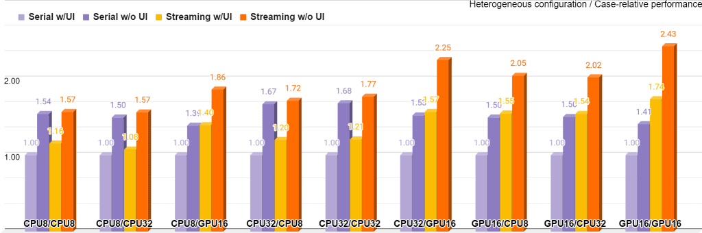
The chart is grouped into nine buckets, where every bucket stands for a target+precision pair for each network. For example, “CPU8/GPU16” means FD runs on CPU with INT8 precision, and LPD runs on GPU with FP16 precision. Every bucket is weighted by its baseline’ execution mode “Serial w/UI”, so in every bucket this mode itself is always at the 1.0 mark. Based on that, every bucket shows how the execution policy improves the performance for this particular bucket only with the given UI setting. Using the streaming mode dramatically improves performance in all buckets, with the most visible effect shown at “GPU16/GPU16” and “CPU32/GPU16” cases.

Figure 9 presents another view on this data, now with all measurements weighted by the “CPU32/CPU32/Serial/UI” baseline:

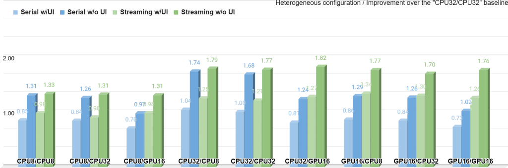
In contrast with the chart in Figure 8, this one reflects how the system’s overall performance changes with the settings. The data is still organized into nine buckets as before, but now it is legit to compare buckets against each other. The overall maximum performance is achieved by the streaming mode with no UI in the “CPU32/GPU16”.

Also it is clear that in the “CPU*/CPU*” cases, the Serial and Streaming performance is nearly the same since all pipeline steps start sharing the same execution resource. This doesn’t apply to the “GPU16/GPU16” case though, as the pipeline still has CPU elements like visualization and decoding, and asynchronous execution of the two networks even at the same GPU has its performance benefits.

Conclusion

Pipelining is a powerful technique that can improve the CV/DL application performance dramatically. OpenCV G-API brings a technological approach to utilizing pipelining in the OpenCV-based user applications, with a compact C++ interface to express pipelines and a complex execution engine under the hood. With this API, the CV/DL application logic becomes decoupled from the way it runs, and the latter becomes configurable with resources managed automatically.

The current pipelining implementation in G-API is still far from ideal, though, but even in its current early state it gives a significant extra throughput compared to the serial mode; further improvements to it are planned in the future OpenCV releases.

Resources

This article refers to a number of online resources, this section lists those for convenience, as well as some additional materials:

1. OpenCV project on GitHub: https://github.com/opencv/opencv
2. OpenVINO™ Open Model Zoo project on GitHub:https://github.com/opencv/open_model_zoo
3. Documentation on OpenCV G-API: https://docs.opencv.org/4.4.0/d0/d1e/gapi.html
4. Tutorials on OpenCV G-API: https://docs.opencv.org/4.4.0/df/d7e/tutorial_table_of_content_gapi.html
5. Slides on OpenCV G-API: https://github.com/opencv/opencv/wiki/files/2020-02-03-GAPI_Overview.pdf 
6. OpenVX™ standard by the Khronos® Group: https://www.khronos.org/registry/OpenVX/
7. OpenVX™ Pipelining extension: https://www.khronos.org/registry/OpenVX/extensions/vx_khr_pipelining/1.1/html/vx_khr_pipelining_1_1_0.html
8. Intel® Threading Building Blocks: https://www.threadingbuildingblocks.org/intel-tbb-tutorial 
9. GStreamer media framework: https://gstreamer.freedesktop.org/ 

The sample video used in this article is “Bus” by sarabernal15 which is available under the CC BY-SA license. Performance measurement script and the sample itself are parts of the OpenCV library.

Legal information

Software and workloads used in performance tests may have been optimized for performance only on Intel microprocessors.  Performance tests, such as SYSmark and MobileMark, are measured using specific computer systems, components, software, operations and functions.  Any change to any of those factors may cause the results to vary.  You should consult other information and performance tests to assist you in fully evaluating your contemplated purchases, including the performance of that product when combined with other products.   For more complete information visit www.intel.com/benchmarks.

Performance results are based on testing as of dates shown in configurations and may not reflect all publicly available security updates.  See backup for configuration details.  No product or component can be absolutely secure. 

Intel’s compilers may or may not optimize to the same degree for non-Intel microprocessors for optimizations that are not unique to Intel microprocessors. These optimizations include SSE2, SSE3, and SSSE3 instruction sets and other optimizations. Intel does not guarantee the availability, functionality, or effectiveness of any optimization on microprocessors not manufactured by Intel. Microprocessor-dependent optimizations in this product are intended for use with Intel microprocessors. Certain optimizations not specific to Intel microarchitecture are reserved for Intel microprocessors. Please refer to the applicable product User and Reference Guides for more information regarding the specific instruction sets covered by this notice.  Notice Revision #20110804

Your costs and results may vary. 

Intel technologies may require enabled hardware, software or service activation.

© Intel Corporation.  Intel, the Intel logo, and other Intel marks are trademarks of Intel Corporation or its subsidiaries.  Other names and brands may be claimed as the property of others.