Imagine a robot rolling through a building, a car driving through city streets, or a drone flying over a campus. Hours later, it reaches a familiar-looking spot and silently asks a crucial question: “Have I been here before?” This deceptively simple question is at the heart of Visual Place Recognition (VPR).
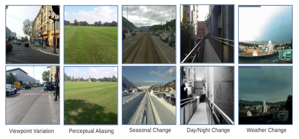
Visual Place Recognition is the task of identifying previously visited locations using only visual input, such as images from a camera, no GPS, no maps, no external sensors. Despite its straightforward appearance, VPR is one of the most challenging and important problems in modern robotics and computer vision. A place might look completely different at night, in the rain, from another angle, or months later in a different season, and yet the system must still recognize it as the same location.
In this blog, we explore Visual Place Recognition (VPR) with hands-on examples using OpenCV and lightweight Python tools. You will create a practical VPR pipeline that includes visual descriptor extraction, global image encoding, similarity-based image retrieval, and optional geometric verification. By the end, you’ll understand how VPR works in practice and have a standalone system capable of detecting revisited places and generating loop-closure candidates.
Table of contents
What is Visual Place Recognition (VPR)?
Visual Place Recognition (VPR) is the process of recognizing a place you’ve visited before using only visual information, such as images or video frames. It enables systems such as robots, drones, and autonomous vehicles to “remember” landmarks, close loops in their maps, and correct positional errors. Unlike GPS, which can fail indoors or in dense urban areas, VPR relies on visual cues and can operate under a wide range of conditions.
VPR must handle appearance changes (day vs. night, seasonal variations, or weather) and viewpoint changes (different angles or perspectives). It is closely related to localization, loop closure, and image retrieval, and is a critical component in many autonomous navigation systems.
The concept of place recognition has existed for decades, but research in visual place recognition has grown rapidly in recent years, driven by improvements in camera hardware and the rise of deep learning-based techniques.
Why is VPR Important?
Visual Place Recognition is not just an academic problem; it is a core capability that enables intelligent machines to function reliably in the real world. Any system that moves through an environment over time must be able to recognize previously visited locations to reason about its current location and its history.
Applications:
VPR is widely used in:
- Autonomous navigation – Self-driving cars and mobile robots use VPR to recognize previously visited roads or indoor spaces, especially when GPS is unreliable.
- SLAM and robotics (loop closure) – VPR helps robots detect revisited locations, enabling loop closure and correcting accumulated localization drift.
- Drone mapping and inspection – Drones use VPR to recognize the same areas across multiple flights, allowing consistent mapping and infrastructure monitoring.
- Augmented reality (AR) systems rely on VPR to anchor virtual content to real-world locations across multiple sessions.
- Image-based place search – VPR enables retrieving the location of a photo by matching it against large visual databases.
Real-World Impact:
In practical systems, errors accumulate over time due to sensor drift and environmental changes. VPR acts as a visual memory, allowing systems to recognize familiar places and correct errors, leading to more robust, long-term autonomy.
Visual bag of Words(BoW)
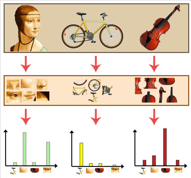
Before the rise of deep learning, one of the most influential ideas in Visual Place Recognition was the Visual Bag-of-Words (BoW) model, an adaptation of the Bag-of-Words concept from text retrieval to images.
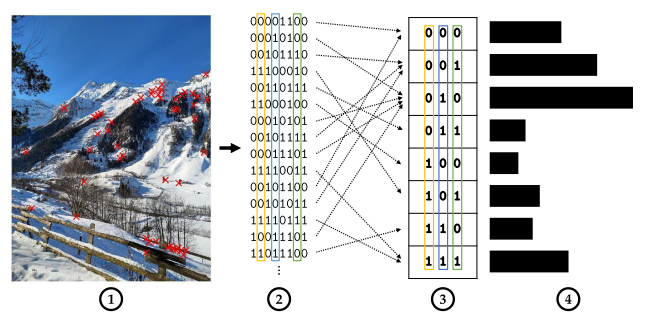
In BoW, an image is treated as an unordered collection of local visual features (such as SIFT, SURF, or ORB). These features are clustered into a fixed number of visual words using techniques like k-means. Each image is then represented as a histogram over these visual words.
How It Works?
- Extract local features(e.g., SIFT, ORB, FAST+BRIEF): For each image, detect keypoints and compute descriptors. In OpenCV, this is typically done with ORB (binary) or SIFT (float).
- Build a visual vocabulary (codebook): Collect descriptors from many images and cluster them (usually k-means). Each cluster center becomes a visual word.
- Assign each feature to the nearest word: Create a histogram (bag of words). An image becomes a list of word IDs
- Use TF-IDF weighting and match histograms: Count how often each word appears. That gives a vector of length K. To improve retrieval quality, you typically apply TF-IDF weighting so that “common” words (e.g., repetitive textures) get downweighted.
- Retrieval: To find the best match for a query image, compute its histogram and compare it to database histograms (cosine similarity / L2 / dot product). You retrieve top-K candidates.
Where BOW fits in VPR
A Visual Bag-of-Words (BoW) enables fast, scalable place retrieval by representing each image as a histogram of visual words. This allows efficient search using inverted files or vocabulary trees, making it suitable for large databases.
When combined with binary features such as ORB or FAST+BRIEF, BoW becomes very fast because matching is performed using the Hamming distance, which is ideal for real-time and resource-limited systems.
Early VPR systems, such as FAB-MAP, used BoW for loop closure detection in SLAM. While modern deep learning methods usually achieve higher accuracy, BoW remains lightweight, interpretable, and easy to implement.
Methods for Visual Place Recognition
VPR methods have evolved from handcrafted to deep learning-based approaches, with a strong emphasis on efficiency for robotics applications. Below are key categories and notable techniques:
Traditional Methods
- Local Feature Matching: Direct matching of keypoints (e.g., ORB, SIFT) with geometric verification (RANSAC). Simple but computationally intensive for large databases.
- Bag of Words (BoW): As above, aggregates local features into global histograms. Variants include DBoW (efficient binary version).
- VLAD and Fisher Vectors: Aggregate residuals or probabilities from local descriptors for more discriminative global representations.
Specific traditional methods include:
DBoW (Distributed Bag of Words): DBoW, often referred to as DBoW2, is an improved hierarchical bag-of-words library implemented in C++ for indexing and converting images into bag-of-words representations. It uses a hierarchical tree to approximate nearest neighbors in the feature space and create a visual vocabulary, enabling fast place recognition in image sequences. DBoW is particularly effective with binary descriptors like ORB and is commonly used in systems like ORB-SLAM for loop closure detection. It supports quick queries and feature comparisons through inverted and direct files.
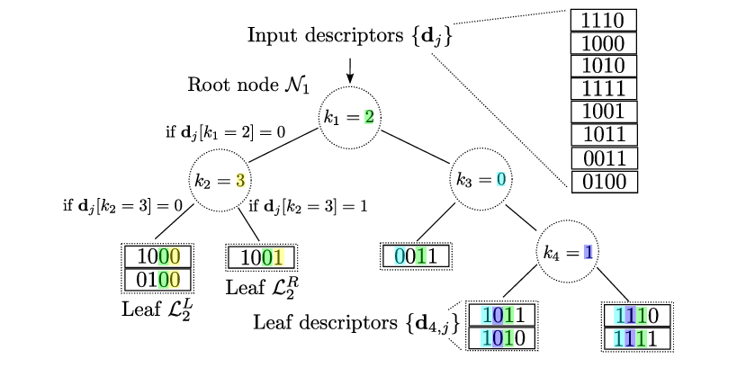
HBST (Hamming Distance Embedding Binary Search Tree): HBST is a method for binary descriptor matching and image retrieval in VPR that embeds descriptors into a binary search tree using Hamming distance. It allows for logarithmic-time search and insertion by exploiting properties of binary features, making it efficient for feature-based place recognition. HBST has been shown to outperform several state-of-the-art methods in comparative experiments on public datasets, particularly in terms of speed and accuracy for binary descriptors.
HashBoW (Hashing-Based Bag of Words): A novel hashing-based approach to bag-of-words for VPR, using locality-sensitive hashing to cluster feature descriptors and treat the resulting hashes as visual words in a BoW model. This method enhances efficiency by avoiding traditional clustering methods such as k-means, making it suitable for accurate, fast place recognition. It has been evaluated in benchmarking suites, showing improvements in retrieval performance for large-scale datasets.
Deep Learning Methods
- CNN-Based: Use pre-trained networks like ResNet for global descriptors. Examples: NetVLAD (end-to-end trainable VLAD layer), MixVPR (feature mixing for robustness).
- Transformer-Based: Leverage attention mechanisms (e.g., ViT or DINOv2) for better handling of long-range dependencies and viewpoint changes.
- Cross-Modal: Combine visuals with LiDAR or semantics (e.g., using a LoST descriptor with semantic segmentation across opposite viewpoints).
- Hybrid: Our scripts blend ORB (handcrafted) with ResNet+GeM (deep), offering a balance of speed and accuracy.
Implementation
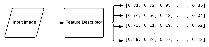
Our VPR pipeline integrates OpenCV with CNN-based global descriptors for practical use. We encode each image into a compact vector. This uses a ResNet50 backbone combined with Generalized Mean (GeM) pooling.
The core task? It’s nearest-neighbor retrieval in descriptor space. We rely on cosine similarity to spot similar past locations.
To cut down false positives:
- Apply similarity thresholds.
- Use temporal filtering to skip nearby frames.
For extra reliability, add optional geometric checks. These involve OpenCV’s ORB features and RANSAC for homography estimation.
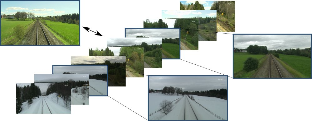
We showcase this on the Nordland dataset, a key VPR benchmark. It features a 728 km Norwegian train route filmed over four seasons: spring, summer, fall, and winter.
Why Nordland? It offers pixel-aligned sequences, perfect for testing against harsh changes such as lighting shifts, weather variations, and seasonal foliage. While Nordland is used in our experiments, the pipeline is not limited to this dataset. Other public benchmarks can be used, or custom datasets can be created. For additional examples, the VPR Datasets Downloader offers convenient access to a wide range of commonly used VPR datasets.
Within the code:
- A fixed database folder set is first processed to compute and store global descriptors
- Query folder images are then processed sequentially and matched against this database
The pipeline operates in an offline retrieval setting, where database and query images are predefined, and matching is performed by comparing each query descriptor against the stored database descriptors.
import cv2
import torch
import torch.nn.functional as F
import numpy as np
from torchvision import models, transforms

# Global descriptor network (ResNet50 + GeM)
class GeM(torch.nn.Module):
    def __init__(self, p=3.0, eps=1e-6):
        super().__init__()
        self.p = torch.nn.Parameter(torch.ones(1) * p)
        self.eps = eps

    def forward(self, x):
        x = x.clamp(min=self.eps).pow(self.p)
        x = F.avg_pool2d(x, (x.size(-2), x.size(-1)))
        return x.pow(1.0 / self.p)

class GlobalDescriptorNet(torch.nn.Module):
    def __init__(self, dim=512):
        super().__init__()
        backbone = models.resnet50(weights="DEFAULT")
        self.features = torch.nn.Sequential(*list(backbone.children())[:-2])
        self.pool = GeM()
        self.proj = torch.nn.Linear(2048, dim)

    def forward(self, x):
        x = self.features(x)
        x = self.pool(x).squeeze(-1).squeeze(-1)
        x = self.proj(x)
        return F.normalize(x, dim=1)

# Descriptor extraction
transform = transforms.Compose([
    transforms.ToPILImage(),
    transforms.Resize(384),
    transforms.CenterCrop(384),
    transforms.ToTensor(),
    transforms.Normalize(
        mean=models.ResNet50_Weights.DEFAULT.transforms().mean,
        std=models.ResNet50_Weights.DEFAULT.transforms().std,
    ),
])


@torch.no_grad()
def extract_descriptor(model, img_bgr, device):
    img_rgb = cv2.cvtColor(img_bgr, cv2.COLOR_BGR2RGB)
    x = transform(img_rgb).unsqueeze(0).to(device)
    return model(x).cpu().numpy().squeeze()


# Optional geometric verification (placeholder)

def geometric_verification(img1, img2):
    # ORB + RANSAC would go here
    return True
# Main retrieval loop (offline VPR)
device = torch.device("cuda" if torch.cuda.is_available() else "cpu")
model = GlobalDescriptorNet().to(device).eval()

query_paths = [...]     # list of query image paths
database_paths = [...]  # list of database image paths

# Encode database once
db_desc = []
for p in database_paths:
    img = cv2.imread(p)
    db_desc.append(extract_descriptor(model, img, device))
db_desc = np.stack(db_desc)

# Query against database
SIM_THRESHOLD = 0.75

for q_path in query_paths:
    q_img = cv2.imread(q_path)
    q_desc = extract_descriptor(model, q_img, device)

    sims = db_desc @ q_desc              # cosine similarity
    best_idx = np.argmax(sims)

    if sims[best_idx] > SIM_THRESHOLD:
        print(f"Match: {q_path} → {database_paths[best_idx]}")
( Full source code is available at the OpenCV Github repository. )
Example run:
- Offline mode: Offline VPR treats place recognition as an image retrieval problem. Given a fixed database of reference images, each query image is independently matched against the entire database to find the most similar location.
python3 VPR.py
--db_dir dataset_root/database
--query_dir dataset_root/query
--output_dir outputs
--verify_geom


[INFO] Offline mode
[INFO] DB images: 248 | Query images: 2226
Encoding DB: 100%|███████████████████████████████████████████████████| 248/248 [00:37<00:00,  6.54it/s]
Querying: 100%|████████████████████████████████████████████████████| 2226/2226 [09:04<00:00,  4.09it/s]
[INFO] Saved results: outputs/loop_closures.json
[INFO] Total accepted matches/loops: 640
[INFO] Saved match previews in: outputs/matches
[INFO] Saved similarity plot: outputs/similarity_plot.png
- Online mode: Images are processed sequentially, and each frame is matched only against previously seen frames. This mirrors real SLAM systems, where future observations are unavailable and loop closures must be detected causally.
python3 VPR.py \
  --images_dir dataset_root/Images/ \
  --output_dir outputs_online \
  --sim_threshold 0.75 \
  --exclude_recent 30 \
  --min_loop_gap 150 \
  --verify_geom


[INFO] Online mode: Found 2474 images.
Processing frames:  14%|██████▎                                     | 35
Processing frames:  14%|██████▎                                     | 35
...
Processing frames:  17%|███████▋                                    |
430/Processing frames: 100%|███████████████████████████████████████████|
2474/2474 [09:55<00:00,  4.16it/s]
[INFO] Saved results: outputs_online/loop_closures.json
[INFO] Total accepted matches/loops: 793
[INFO] Saved match previews in: outputs_online/matches
[INFO] Saved similarity plot: outputs_online/similarity_plot.png
Understanding the Outputs
This Visual Place Recognition (VPR) pipeline produces three complementary outputs. Let’s break them down one by one:
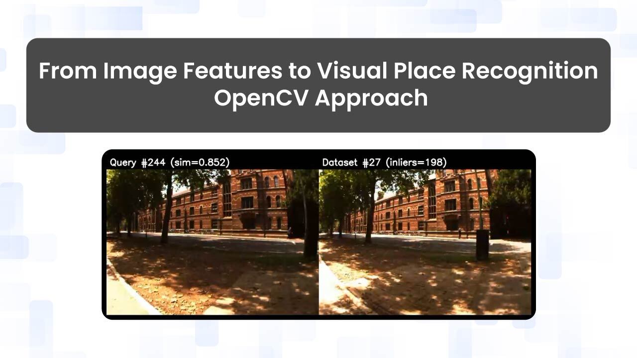
1. Match Visualization Images (outputs/matches/)
Each image in the matches/ folder shows a detected loop closure


Offline output:
Online output:
What you are seeing
- Left image: current frame (query image)
- Right image: previously visited frame (matched image)
- Overlay text:
- Query #7 → index of the current frame
- Match #1 → index of the matched past frame
- score → cosine similarity between global descriptors
- inliers → number of geometrically consistent feature matches
Why this matters
Even though frames are captured far apart in time, the system correctly recognizes that:
- The same physical place has been revisited
- Appearance may differ slightly (viewpoint, lighting)
- The match is not accidental
This is exactly what loop closure detection is supposed to do in SLAM.
2. Loop Closures JSON
The file logs accepted matches in a structured format. It’s an array of objects, each detailing a detection.
{
  "query_idx": 7,
  "match_idx": 1,
  "score": 0.8679320812225342,
  "geom_verified": true,
  "inliers": 52,
  "query_path": "dataset_root/query/0009.jpg",
  "match_path": "dataset_root/database/0011.jpg"
}
Structure and fields:
- query_idx: Index of the current frame
- match_idx: Index of the matched past frame
- score: Cosine similarity of global descriptors
- geom_verified: Passed ORB + RANSAC geometric check
- inliers: Number of consistent feature matches
- query_path, match_path: Path to current image
How to interpret values
- High score (0.84–0.90) → strong global appearance similarity
- Geom verified = true → not a false positive
- Inliers > 20 → spatial layout is consistent
3. Similarity Plot
The generated plot visualized cosine similarities over query indices.
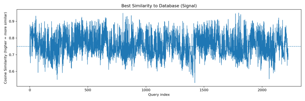
What it shows: Each point represents the highest similarity score for a query against the database. Higher values indicate stronger potential matches.
Threshold line: A dashed horizontal line at 0.75 (default) marks the acceptance cutoff. Peaks above this suggest detected loops or revisits.
Patterns observed: Similarities range from ~0.6 to ~0.9. Lower scores at the beginning and end correspond to unique scenes, while mid-sequence peaks (e.g., indices 500–1500) reflect repetitive environments such as tunnels or stations.
How to read the plot
- Flat low region → no loop closures (new environment)
- Sharp peaks above threshold → revisiting known places
- Clusters of peaks → sustained revisit of the same location
This plot is often called a loop-closure signal in the SLAM literature.
How Visual Place Recognition Fits Into SLAM
In a full SLAM (Simultaneous Localization and Mapping) system, Visual Place Recognition typically serves as the loop closure proposal mechanism rather than the final decision-maker. As the robot explores an environment, VPR continuously compares the current camera frame against previously stored images to identify potential revisits. When a strong match is detected, the system proposes a loop closure candidate. This candidate is then passed to the SLAM backend, which performs pose-graph optimization to verify and integrate the loop-closure constraint. If accepted, the optimization step corrects accumulated drift in the robot’s estimated trajectory and map. In this sense, VPR provides the “memory” needed to recognize familiar places, while SLAM handles global consistency and map correction over time.

Limitations and Challenges in VPR
Despite strong performance in many environments, Visual Place Recognition systems face several important limitations:
- Perceptual aliasing remains a major issue, where different locations with similar visual structures, such as corridors or building facades, lead to false matches.
- VPR is also sensitive to appearance changes caused by viewpoint shifts, direction of travel, lighting, weather, and seasonal variations, which can reduce descriptor similarity or break geometric verification.
- Additionally, dynamic objects like people and vehicles can dominate local features, lowering the number of reliable inliers.
These limitations impact both matching accuracy and scalability, highlighting the need for more invariant representations and robust verification strategies.
Conclusion
Visual Place Recognition enables intelligent systems to recognize previously visited locations and is a core component of long-term autonomy. In this blog, we built a practical VPR pipeline using OpenCV and modern deep learning, progressing from raw images to reliable loop-closure detection.
By combining CNN-based global descriptors with cosine similarity retrieval and lightweight geometric verification using ORB and RANSAC, we achieved a system that is both efficient and robust, closely mirroring real-world SLAM pipelines.
This work shows that effective VPR does not require complex training pipelines or large infrastructure. With a clear design and standard datasets, it is possible to build an accurate, extensible VPR system suitable for image retrieval, loop closure, or integration into full SLAM frameworks.
Reference
Visual Place Recognition: A Hands-on Tutorial
Norland Dataset – Hugging Face
Visual place recognition: A survey from deep learning perspective


5K+ Learners
Join Free VLM Bootcamp3 Hours of Learning