In computer vision, detecting blobs(regions) that differ from their surroundings is a common and powerful technique. A blob can be as simple as a spot of light in an image or as complex as a moving object in a video. Blob detection is crucial in various domains such as microscopy, surveillance, object tracking, astronomy, and medical imaging. In this article, we will understand the theoretical concepts and mathematical foundations behind blob detection, implement blob detection using OpenCV’s SimpleBlobDetector in Python and C++ and explore parameter tuning and alternate approaches like contours and connected components

Import cv2

Before using any OpenCV functions, we must first import the library. This is the essential first step to access all OpenCV functionalities.

Python

# import the cv2 library
import cv2

C++

//Include Libraries
//OpenCV's cv::Mat acts like NumPy arrays for image processing.

#include<opencv2/opencv.hpp>
#include<iostream>

We are assuming  that you have already installed OpenCV on your device.
If not please refer the relevant links below:

• Install OpenCV on Windows
• Install OpenCV on MacOS
• Install OpenCV on Ubuntu

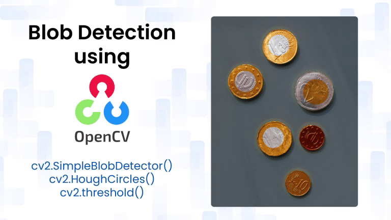
Example Image

What is a Blob?

A blob is a region in an image where some properties—such as intensity or color—are uniform or vary within a defined range. Blobs are usually visually distinguishable structures like:

• Bright or dark spots
• Regions of uniform color or texture
• Objects with approximately circular or elliptical shapes

In simpler terms, blobs are groupings of connected pixels that we consider as one unit of information.

How does Blob detection work ?

SimpleBlobDetector, as the name implies, is based on a rather simple algorithm described below. The algorithm is controlled by parameters ( shown in bold below )  and has the following steps. 

1. Thresholding : Convert the source images to several binary images by thresholding the source image with thresholds starting at minThreshold. These thresholds are incremented  by thresholdStep until maxThreshold. So the first threshold is minThreshold, the second is minThreshold + thresholdStep, the third is minThreshold + 2 x thresholdStep, and so on.
2. Grouping : In each binary image,  connected white pixels are grouped together.  Let’s call these binary blobs.
3. Merging : The centers of the binary blobs in the binary images are computed, and  blobs located closer than minDistBetweenBlobs are merged.
4. Center & Radius Calculation :  The centers and radii of the new merged blobs are computed and returned.

Filtering Blobs

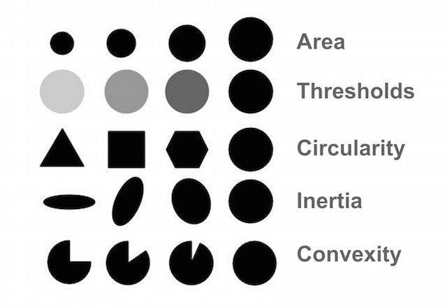
The parameters for SimpleBlobDetector can be set to filter the type of blobs we want.

• By Color : First you need to set filterByColor = 1. Set blobColor = 0 to select darker blobs, and blobColor = 255 for lighter blobs. 
• By Size :  You can filter the blobs based on size by setting the parameters filterByArea = 1, and appropriate values for minArea and maxArea. E.g. setting minArea = 100 will filter out all the blobs that have less than 100 pixels.
• By Shape : Now shape has three different parameters.
• Circularity :  This just measures how close to a circle the blob is. E.g. a regular hexagon has higher circularity than, say, a square. To filter by circularity, set filterByCircularity = 1.  Then set appropriate values for minCircularity and maxCircularity.
• This means that a typical circle has a circularity of 1, whereas the circularity of a square is 0.785, and so on.
• Convexity : Convexity is defined as the (Area of the Blob / Area of its convex hull). Now, the convex Hull of a shape is the tightest convex shape that completely encloses the shape. To filter by convexity, set filterByConvexity = 1, followed by setting 0 ≤ minConvexity ≤ 1 and maxConvexity ( ≤ 1) 
• Inertia Ratio : Don’t let this scare you. Mathematicians often use confusing words to describe something very simple. All you have to know is that this measures how elongated a shape is. E.g. For a circle, this value is 1, for an ellipse it is between 0 and 1, and for a line it is 0. To filter by inertia ratio, set filterByInertia = 1, and set 0 ≤ minInertiaRatio ≤ 1 and maxInertiaRatio (≤ 1 ) appropriately.

Techniques for Blob Detection

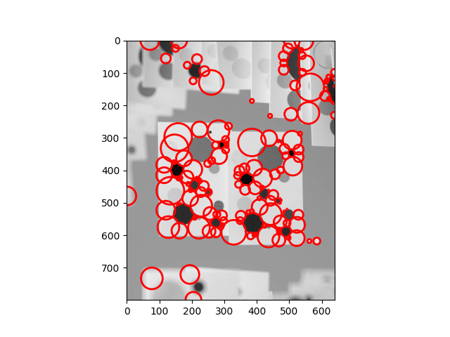
Laplacian of Gaussian (LoG)

The Laplacian of Gaussian is a classical blob detector. The image is smoothed using a Gaussian kernel and then filtered using the Laplacian operator (second derivative).

• G(x,y,σ): Gaussian function with standard deviation σ
• ∇2: Laplacian operator
• I(x,y): Input image
  

Although the LoG approach can identify blobs of different sizes effectively, it may return multiple strong responses for a single blob. Often post-processing techniques like non-maximum suppression are applied to keep only the strongest response for each blob and eliminate duplicates.

Python

from skimage import feature, color, io
import matplotlib.pyplot as plt

image = color.rgb2gray(io.imread("example image.jpg"))
blobs_log = feature.blob_log(image, max_sigma=30, num_sigma=10, threshold=0.1)

# Compute radii
blobs_log[:, 2] = blobs_log[:, 2] * (2 ** 0.5)

# Display
fig, ax = plt.subplots()
ax.imshow(image, cmap='gray')
for y, x, r in blobs_log:
    c = plt.Circle((x, y), r, color='red', linewidth=2, fill=False)
    ax.add_patch(c)
plt.show()

C++

#include <opencv2/opencv.hpp>
using namespace cv;
int main() {
    Mat image = imread("example.jpg", IMREAD_GRAYSCALE);
    if (image.empty()) return -1;

    // Apply Gaussian blur
    Mat blurred;
    GaussianBlur(image, blurred, Size(0, 0), 2);

    // Apply Laplacian
    Mat laplacian;
    Laplacian(blurred, laplacian, CV_64F);

    // Convert to displayable format
    Mat result;
    convertScaleAbs(laplacian, result);
    imshow("LoG Blobs", result);
    imwrite("log_blobs.jpg", result);

    waitKey(0);
    return 0;
}

• The image is first smoothed with a Gaussian filter to reduce noise.
• The Laplacian operator is applied to detect regions with sharp intensity changes (blobs).

Output

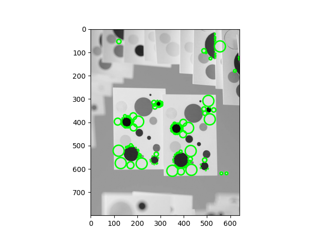
Difference of Gaussian (DoG)

This is an approximation of LoG and is computationally more efficient.The DoG algorithm computes the difference between two Gaussian-smoothed pictures. It is handy for recognizing blobs of a given size range. We can vary the standard deviation of the Gaussian kernels to control the size of the detected blobs.

• k: scale multiplication factor

Python

from skimage import feature, color, io
import matplotlib.pyplot as plt

image = color.rgb2gray(io.imread("example image.jpg"))
blobs_dog = feature.blob_dog(image, max_sigma=30, threshold=0.1)

# Compute radii
blobs_dog[:, 2] = blobs_dog[:, 2] * (2 ** 0.5)

# Display
fig, ax = plt.subplots()
ax.imshow(image, cmap='gray')
for y, x, r in blobs_dog:
    c = plt.Circle((x, y), r, color='lime', linewidth=2, fill=False)
    ax.add_patch(c)
plt.show()

C++

#include <opencv2/opencv.hpp>
using namespace cv;
int main() {
    Mat image = imread("example.jpg", IMREAD_GRAYSCALE);
    if (image.empty()) return -1;

    // Apply two Gaussian blurs with different sigmas
    Mat g1, g2, dog;
    GaussianBlur(image, g1, Size(0, 0), 1);
    GaussianBlur(image, g2, Size(0, 0), 2);

    // Subtract to get DoG
    subtract(g1, g2, dog);

    // Convert to displayable format
    Mat result;
    normalize(dog, result, 0, 255, NORM_MINMAX);
    result.convertTo(result, CV_8U);
    imshow("DoG Blobs", result);
    imwrite("dog_blobs.jpg", result);

    waitKey(0);
    return 0;
}

• Two Gaussian blurs with different σ values are applied.
• Their difference highlights structures (blobs) that vary at specific scales.

Output

Determinant of Hessian (DoH)

Focuses on second-order derivatives and looks for strong curvature changes. Blobs are identified via the DoH approach by using the determinant of the Hessian matrix. The local curvature of an image is represented by the Hessian matrix. The local maxima in the Hessian’s determinant can be used to locate blobs of various sizes and forms.

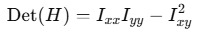
• Where Ixx, Iyy, Ixy are second-order partial derivatives
  

Python

from skimage import feature, color, io
import matplotlib.pyplot as plt

image = color.rgb2gray(io.imread("example image.jpg"))
blobs_doh = feature.blob_doh(image, max_sigma=30, threshold=0.01)

# Display
fig, ax = plt.subplots()
ax.imshow(image, cmap='gray')
for y, x, r in blobs_doh:
    c = plt.Circle((x, y), r, color='blue', linewidth=2, fill=False)
    ax.add_patch(c)
plt.show()

C++

#include <opencv2/opencv.hpp>
using namespace cv;
int main() {
    Mat image = imread("example.jpg", IMREAD_GRAYSCALE);
    if (image.empty()) return -1;

    // Compute second-order derivatives
    Mat dxx, dyy, dxy;
    Sobel(image, dxx, CV_64F, 2, 0);
    Sobel(image, dyy, CV_64F, 0, 2);
    Sobel(image, dxy, CV_64F, 1, 1);

    // Determinant of Hessian
    Mat hessianDet = dxx.mul(dyy) - dxy.mul(dxy);

    // Normalize and convert to displayable format
    Mat result;
    normalize(hessianDet, result, 0, 255, NORM_MINMAX);
    result.convertTo(result, CV_8U);
    imshow("DoH Blobs", result);
    imwrite("doh_blobs.jpg", result);

    waitKey(0);
    return 0;
}

• Second-order Sobel derivatives are computed to approximate the Hessian matrix.
• The determinant of the Hessian highlights blob-like structures where curvature is high.

Output

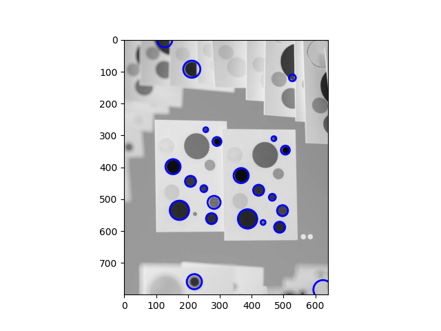
OpenCV’s SimpleBlobDetector

OpenCV wraps blob detection in the SimpleBlobDetector class. It detects blobs by analyzing connected regions and filtering based on shape, size, and intensity characteristics.

Python

detector = cv2.SimpleBlobDetector_create(params)

C++

cv::Ptr<cv::SimpleBlobDetector> detector = cv::SimpleBlobDetector::create(params);

params: An instance of cv2.SimpleBlobDetector_Params() containing configuration options.

We set these using the Params object before calling create().

• minThreshold: Lower threshold for the internal binary thresholding (default: 50)
• maxThreshold: Upper threshold for binary thresholding (default: 220)
• thresholdStep: Step size between thresholds (default: 10)
• filterByColor: Enable/disable color filtering (default: true)
• blobColor: Blob color to detect (0 for dark, 255 for bright blobs)
• filterByArea: Enable area-based filtering (default: true)
• minArea: Minimum area of blobs (default: 25)
• maxArea: Maximum area of blobs (default: 5000)
• filterByCircularity: Enable filtering based on circularity (default: false)
• minCircularity: Minimum circularity (0.0 to 1.0)
• maxCircularity: Maximum circularity
• filterByInertia: Enable filtering based on elongation (default: true)
• minInertiaRatio: Ratio of minimum inertia (default: 0.1)
• maxInertiaRatio: Maximum inertia ratio
• filterByConvexity: Enable filtering based on convexity (default: true)
• minConvexity: Minimum convexity (default: 0.95)
• maxConvexity: Maximum convexity

All these parameters are set using the params object before calling create(params).

Implementation

Python

import cv2
import numpy as np

# Load image
image = cv2.imread("example image.jpg", cv2.IMREAD_GRAYSCALE)

# Setup SimpleBlobDetector parameters
params = cv2.SimpleBlobDetector_Params()

# Thresholds for binarization
params.minThreshold = 10
params.maxThreshold = 200

# Filter by Area
params.filterByArea = True
params.minArea = 10

# Filter by Circularity
params.filterByCircularity = True
params.minCircularity = 0.1

# Filter by Convexity
params.filterByConvexity = True
params.minConvexity = 0.87

# Filter by Inertia
params.filterByInertia = True
params.minInertiaRatio = 0.01

# Create a detector with the parameters
detector = cv2.SimpleBlobDetector_create(params)

# Detect blobs
keypoints = detector.detect(image)

# Draw blobs as red circles
output = cv2.drawKeypoints(image, keypoints, np.array([]), (0, 0, 255),
                           cv2.DRAW_MATCHES_FLAGS_DRAW_RICH_KEYPOINTS)

# Show the output
cv2.imshow("Blobs Detected", output)
cv2.waitKey(0)
cv2.destroyAllWindows()

C++

#include <opencv2/opencv.hpp>
#include <opencv2/features2d.hpp>

int main() {
    cv::Mat image = cv::imread("blobs.jpg", cv::IMREAD_GRAYSCALE);

    // Set up parameters
    cv::SimpleBlobDetector::Params params;
    params.minThreshold = 10;
    params.maxThreshold = 200;
    params.filterByArea = true;
    params.minArea = 10;
    params.filterByCircularity = true;
    params.minCircularity = 0.1;
    params.filterByConvexity = true;
    params.minConvexity = 0.87;
    params.filterByInertia = true;
    params.minInertiaRatio = 0.01;

    // Create detector and detect blobs
    cv::Ptr<cv::SimpleBlobDetector> detector = cv::SimpleBlobDetector::create(params);
    std::vector<cv::KeyPoint> keypoints;
    detector->detect(image, keypoints);

    // Draw the keypoints
    cv::Mat output;
    cv::drawKeypoints(image, keypoints, output, cv::Scalar(0, 0, 255),
                      cv::DrawMatchesFlags::DRAW_RICH_KEYPOINTS);

    // Display result
    cv::imshow("Blobs Detected", output);
    cv::waitKey(0);
    return 0;
}

Output

Applications of Blob Detection

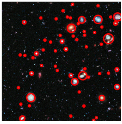
• Astronomy: Blob detection is widely used in astronomical imaging to identify stars, galaxies, and other celestial objects. These objects typically appear as bright blobs on a dark background, making them ideal candidates for detection using intensity-based blob detectors.

Source

• Microscopy: In biological and medical microscopy, blob detection helps in identifying cells, bacteria, or other microorganisms. Since these entities often have circular or elliptical shapes and differ in intensity from their surroundings, blob detection provides a straightforward method for segmentation and counting.

Source

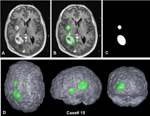
• Medical Imaging: Blob detection techniques can be employed to locate abnormalities such as tumors, cysts, or lesions in scans like MRIs or CTs. These irregular growths often manifest as isolated regions with distinct texture or brightness, making blob detectors valuable in diagnostic imaging.

Source

• Industrial Automation: In manufacturing and assembly lines, blob detection helps recognize and track specific parts on conveyor belts. Whether it’s identifying missing components or verifying the presence of correctly shaped items, blob detectors assist in quality control and robotic vision.

Source

Summary

This blog explored the concept and implementation of blob detection, a computer vision technique used to identify regions in an image that differed in brightness or texture compared to surrounding areas. It introduced OpenCV’s SimpleBlobDetector, explained its internal filtering mechanisms such as area, circularity, convexity, inertia, and color. Readers learned how to configure detection parameters using the SimpleBlobDetector_Params object in both Python and C++, with a breakdown of each parameter’s purpose and effect.

Blob detection was presented as a cornerstone technique in image analysis and computer vision. OpenCV’s SimpleBlobDetector served as a flexible and efficient way to detect regions of interest based on geometric and intensity features. By understanding the theory, adjusting detector parameters, and experimenting with alternate methods like contours or connected components, readers were equipped to apply blob detection across a wide range of practical applications.