Edge detection is a crucial technique in image processing and computer vision, used to identify sharp changes in brightness that typically signify object boundaries, edges, lines, or textures. It enables applications like object recognition, image segmentation, and tracking by highlighting the structural features of an image. In this blog, we’ll explore three of the most popular edge detection methods—Sobel, Laplacian, and Canny—explaining their conceptual foundations, mathematical formulations, and convolution kernels. We’ll also provide complete OpenCV implementations in both Python and C++, so you can easily integrate these techniques into your own projects. Whether you’re processing images for analysis or building a vision-based application, understanding edge detection is essential.

Import cv2

Before using any OpenCV functions, we must first import the library. This is the essential first step to access all OpenCV functionalities.

Python

# import the cv2 library
import cv2

C++

//Include Libraries
//OpenCV's cv::Mat acts like NumPy arrays for image processing.

#include<opencv2/opencv.hpp>
#include<iostream>

We are assuming  that you have already installed OpenCV on your device.
If not please refer the relevant links below:

• Install OpenCV on Windows
• Install OpenCV on MacOS
• Install OpenCV on Ubuntu

Example Image

Understanding Edges in Images

An edge in an image represents a boundary where there is a significant change in intensity or color. Edge detection is crucial for understanding the structure and features within an image, aiding in tasks like object recognition, segmentation, and tracking. Edges are typically detected by identifying areas with high intensity gradients, which can be achieved using various operators that compute derivatives of the image intensity function.

Edges are boundaries between different regions in an image. These are typically caused by:

• Object boundaries
• Surface orientation changes
• Texture changes
• Lighting variations
  

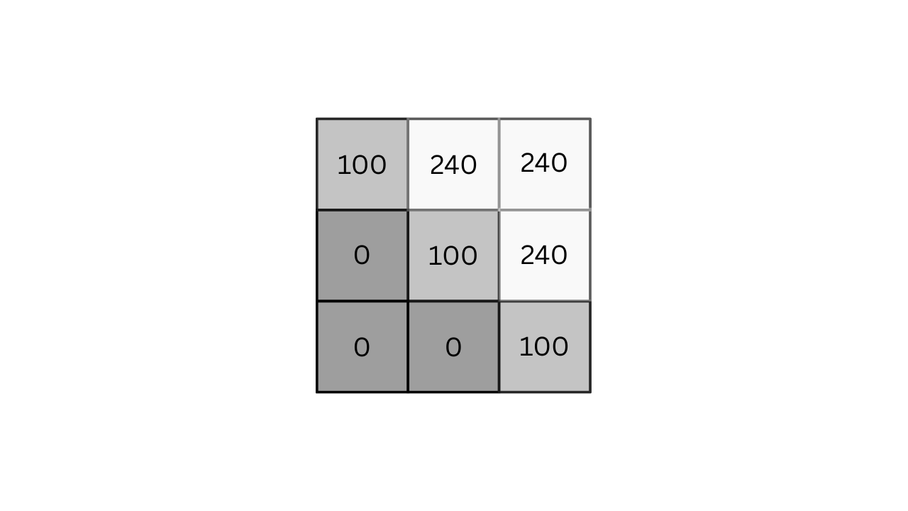
In grayscale images, an edge represents a rapid change in intensity, such as a shift from dark to light within a small number of pixels. This transition is mathematically captured using gradients, which measure changes in pixel intensity. In the image above, the noticeable transition of pixel values from 0 to 240 indicates a significant intensity change. It’s evident that the pixels with a value of 100 correspond to the edge pixels.

In color images, edges are not as straightforward to identify as in grayscale images because each pixel contains multiple channels (typically Red, Green, and Blue), not just a single intensity value. To detect edges in color images, we typically convert the image to a color space where the intensity and color information are more easily separable or we compute gradients in each channel separately.

Color images are often converted to grayscale before applying edge detection techniques like Canny, Sobel, or Laplacian. This simplifies the process by reducing the image to a single intensity channel, making it easier to detect edges based on intensity changes. Once converted to grayscale, these algorithms can effectively highlight the edges in the image.

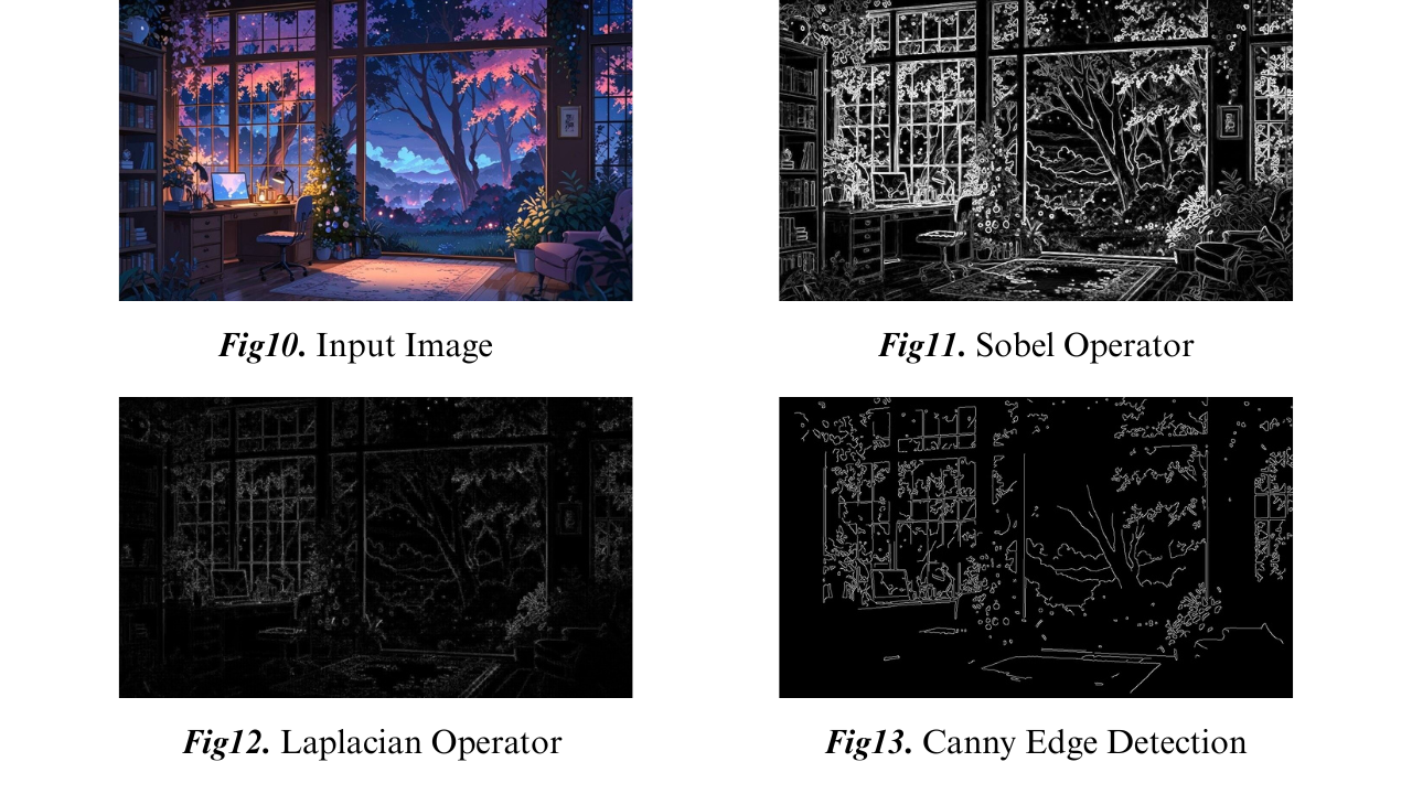
Sobel Operator

The Sobel operator is a discrete differentiation operator that computes an approximation of the gradient of the image intensity function. It emphasizes edge detection in both horizontal and vertical directions by combining Gaussian smoothing and differentiation, making it less sensitive to noise.

Mathematical Formulation

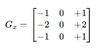
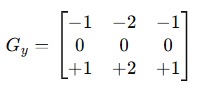
The Sobel operator uses two 3×3 kernels:

• Gx (horizontal changes):

• Gy (vertical changes):

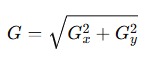
The gradient magnitude is computed as:

Or an approximation:

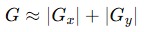
When the Sobel kernel is applied to a region of the image, it performs a convolution operation that emphasizes regions with high spatial frequency, which correspond to edges. For example, applying the Gx kernel will highlight vertical edges, while Gy will highlight horizontal edges.

Python

sobelx = cv2.Sobel(src, ddepth, dx, dy, ksize=3)

C++

Sobel(src, dst, ddepth, dx, dy, ksize);

It accepts the following arguments:

• src: Input image (should be grayscale for edge detection).
• dst (C++ only): Output image where the result is stored.
• ddepth: Desired depth of the output image (e.g., CV_64F allows negative gradients).
• dx: Order of the derivative in the x-direction (set to 1 to detect horizontal changes).
• dy: Order of the derivative in the y-direction (set to 1 to detect vertical changes).
• ksize: Size of the extended Sobel kernel (must be odd: 1, 3, 5, 7; use 1 for Scharr operator).

This syntax applies to detecting gradients in specific directions (horizontal or vertical) using the Sobel operator.

OpenCV Implementation

Python

import cv2
import numpy as np

# Load image in grayscale
img = cv2.imread('exampleimage.JPG', cv2.IMREAD_GRAYSCALE)

# Apply Sobel operator
sobelx = cv2.Sobel(img, cv2.CV_64F, 1, 0, ksize=3)  # Horizontal edges
sobely = cv2.Sobel(img, cv2.CV_64F, 0, 1, ksize=3)  # Vertical edges

# Compute gradient magnitude
gradient_magnitude = cv2.magnitude(sobelx, sobely)

# Convert to uint8
gradient_magnitude = cv2.convertScaleAbs(gradient_magnitude)

# Display result
cv2.imshow("Sobel Edge Detection", gradient_magnitude)

cv2.waitKey(0)
cv2.destroyAllWindows()

C++

#include <opencv2/opencv.hpp>
int main() {
    cv::Mat img = cv::imread("image.jpg", cv::IMREAD_GRAYSCALE);
    if (img.empty()) return -1;
    cv::Mat sobelx, sobely, gradient;

    // Apply Sobel operator
    cv::Sobel(img, sobelx, CV_64F, 1, 0, 3);
    cv::Sobel(img, sobely, CV_64F, 0, 1, 3);

    // Compute gradient magnitude
    cv::magnitude(sobelx, sobely, gradient);

    // Convert to 8-bit image
    cv::Mat gradient_abs;
    cv::convertScaleAbs(gradient, gradient_abs);

    // Display result
    cv::imshow("Sobel Edge Detection", gradient_abs);

    cv::waitKey(0);
    return 0;
}

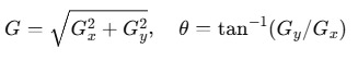
First, the image is loaded in grayscale since edge detection operates on intensity values, not color. Then, the Sobel operator is applied twice — once with dx=1, dy=0 to detect horizontal edges (changes along the x-direction), and once with dx=0, dy=1 for vertical edges (changes along the y-direction). These produce two gradient images: sobelx and sobely.

Next, cv2.magnitude() (or cv::magnitude() in C++) computes the gradient magnitude, which combines the horizontal and vertical components using the formula √(Gx² + Gy²). This gives the overall edge strength at each pixel.

Since the result is in floating-point format, it’s converted to an 8-bit unsigned format using convertScaleAbs() so it can be displayed or saved properly.

Output

Laplacian Operator

The Laplacian operator is a second-order derivative operator that highlights regions of rapid intensity change, effective in edge detection. Unlike Sobel, which is directional, the Laplacian is non-directional and detects edges in all directions.

Mathematical Formulation

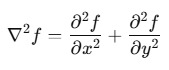
The Laplacian operator is defined as:

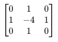
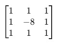
Common kernels:

• 4-neighbor kernel:

• 8-neighbor kernel:

The Laplacian operator, often denoted as Δ or ∇², is a differential operator used in mathematics and physics to calculate the second spatial derivative of a scalar function. It essentially measures the rate of change of the rate of change of a function across its spatial domain. In simpler terms, it indicates how much the function’s value deviates from the average value of its surrounding points. 

Python

laplacian = cv2.Laplacian(src, ddepth, ksize=3)

C++

Laplacian(src, dst, ddepth, ksize);

It accepts the following arguments:

• src: Input image (usually in grayscale).
• dst (C++ only): Output image to store the Laplacian result.
• ddepth: Desired depth of the output image (e.g., CV_64F to capture negative values).
• ksize: Size of the Laplacian kernel (must be odd and positive; typically 1, 3, 5, or 7). Use ksize=1 to apply a 3×3 kernel without scaling.

OpenCV Implementation

Python

import cv2
import numpy as np

# Load image in grayscale
img = cv2.imread('exampleimage.JPG', cv2.IMREAD_GRAYSCALE)

# Apply Laplacian operator
laplacian = cv2.Laplacian(img, cv2.CV_64F)

# Convert to uint8
laplacian_abs = cv2.convertScaleAbs(laplacian)

# Display result
cv2.imshow("Laplacian Edge Detection", laplacian_abs)

cv2.waitKey(0)
cv2.destroyAllWindows()

C++

#include <opencv2/opencv.hpp>
int main() {
    cv::Mat img = cv::imread("image.jpg", cv::IMREAD_GRAYSCALE);
    if (img.empty()) return -1;
    cv::Mat laplacian;

    // Apply Laplacian operator
    cv::Laplacian(img, laplacian, CV_64F);

    // Convert to 8-bit image
    cv::Mat laplacian_abs;
    cv::convertScaleAbs(laplacian, laplacian_abs);

    // Display result
    cv::imshow("Laplacian Edge Detection", laplacian_abs);

    cv::waitKey(0);
    return 0;
}

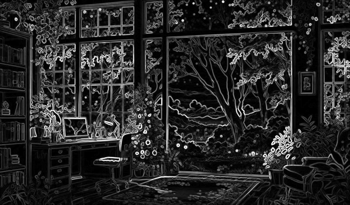
The Laplacian operator is applied, which calculates the second-order derivative of the image to detect areas where the intensity changes rapidly in any direction—these areas correspond to edges. Since the Laplacian output includes negative values (indicating direction of change), it’s converted to an absolute 8-bit format using convertScaleAbs to make it visually displayable.

Output

Canny Edge Detector

The Canny edge detector was developed by John Canny in 1986 and is still one of the most reliable edge detection algorithms. It combines gradient-based edge detection with advanced logic to ensure that the detected edges are thin, connected, and free from noise. Canny Edge Detection is one of the most popular edge-detection methods in use today because it is so robust and flexible. The algorithm itself follows a three-stage process for extracting edges from an image. Add to it image blurring, a necessary preprocessing step to reduce noise. This makes it a four-stage process, which includes:

1. Noise Reduction
2. Calculating the Intensity Gradient of the Image
3. Suppression of False Edges
4. Hysteresis Thresholding

We first convert the image into grayscale.

Noise Reduction

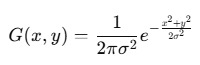
Raw image pixels can often lead to noisy edges, so it is essential to reduce noise before computing edges In Canny Edge Detection, a Gaussian blur filter is used to essentially remove or minimize unnecessary detail that could lead to undesirable edges. Have a look at the image below; Gaussian blur has been applied to the image. As you can see, it appears slightly blurred but still retains a significant amount of detail from which edges can be computed.

Calculating the Intensity Gradient of the Image

Once the image has been smoothed (blurred), it is filtered with a Sobel kernel, both horizontally and vertically. The results from these filtering operations are then used to calculate both the intensity gradient magnitude, and the direction for each pixel. The gradient direction is then rounded to the nearest 45-degree angle.

Suppression of False Edges

After reducing noise and calculating the intensity gradient, the algorithm in this step uses a technique called non-maximum suppression of edges to filter out unwanted pixels (which may not actually constitute an edge). To accomplish this, each pixel is compared to its neighboring pixels in the positive and negative gradient direction. If the gradient magnitude of the current pixel is greater than its neighboring pixels, it is left unchanged. Otherwise, the magnitude of the current pixel is set to zero. The following image illustrates an example.  As you can see, numerous ‘edges’ associated with the image have been significantly subdued.

Hysteresis Thresholding

In this final step of Canny Edge Detection, the gradient magnitudes are compared with two threshold values, one smaller than the other. 

1. If the gradient magnitude value is higher than the larger threshold value, those pixels are associated with solid edges and are included in the final edge map.
2. If the gradient magnitude values are lower than the smaller threshold value, the pixels are suppressed and excluded from the final edge map.
3. All the other pixels, whose gradient magnitudes fall between these two thresholds, are marked as ‘weak’ edges (i.e. they become candidates for being included in the final edge map). 
4. If the ‘weak’ pixels are connected to those associated with solid edges, they are also included in the final edge map. 

Python

edges = cv2.Canny(image, threshold1, threshold2)

C++

Canny(image, edges, threshold1, threshold2);

It accepts the below arguments:

• image: Input image (must be in grayscale).
• edges (C++ only): Output image where edges will be marked as white (255) on a black background.
• threshold1: Lower boundary for the hysteresis thresholding.
• threshold2: Upper boundary for the hysteresis thresholding.

OpenCV Implementation

Python

import cv2

# Load image in grayscale
img = cv2.imread("exampleimage.JPG", cv2.IMREAD_GRAYSCALE)

# Apply Gaussian Blur to reduce noise
blur = cv2.GaussianBlur(img, (5, 5), 1.4)

# Apply Canny Edge Detector
edges = cv2.Canny(blur, threshold1=100, threshold2=200)

# Display result
cv2.imshow("Canny Edge Detection", edges)

cv2.waitKey(0)
cv2.destroyAllWindows()

C++

#include <opencv2/opencv.hpp>
int main() {
    cv::Mat img = cv::imread("image.jpg", cv::IMREAD_GRAYSCALE);
    if (img.empty()) return -1;
    cv::Mat blur, edges;

    // Apply Gaussian blur
    cv::GaussianBlur(img, blur, cv::Size(5, 5), 1.4);

    // Apply Canny Edge Detector
    cv::Canny(blur, edges, 100, 200);

    // Display result
    cv::imshow("Canny Edge Detection", edges);

    cv::waitKey(0);
    return 0;
}

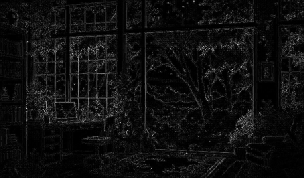
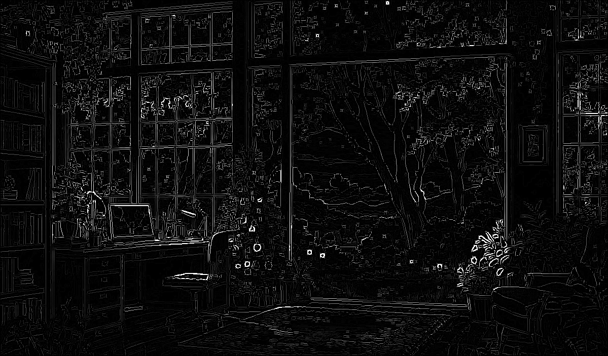
The image is first read in grayscale using cv2.imread(…, cv2.IMREAD_GRAYSCALE) in Python and cv::imread(…, cv::IMREAD_GRAYSCALE) in C++. Grayscale simplifies processing since edge detection relies on intensity changes rather than color. Then a Gaussian blur is applied using cv2.GaussianBlur() in Python and cv::GaussianBlur() in C++. This step reduces noise and smoothens the image to prevent false edges. Next, the Canny edge detector is applied with thresholds 100 and 200 using cv2.Canny() and cv::Canny(), which detects edges by computing gradients and applying non-maximum suppression followed by hysteresis thresholding.

Output

Summary

In this blog, we explored the fundamentals of edge detection, focusing on how edges represent rapid intensity changes in images and why grayscale conversion is essential for simplifying the process. We covered key edge detection techniques like Sobel, which uses first-order derivatives to highlight directional gradients, and the Laplacian operator, which uses second-order derivatives to capture edges in all directions. We also delved into the Canny edge detector, a robust multi-step method that includes blurring, gradient calculation, non-maximum suppression, and hysteresis thresholding. Practical Python and C++ code implementations were provided for each method, along with steps to save intermediate results for visualization.