Autofocus plays a crucial role in imaging systems, ensuring that captured images and video frames are sharp and well-defined. In various applications, such as medical imaging, surveillance, and photography, selecting the sharpest frame from a sequence can significantly enhance the quality of analysis and presentation. In this article, we explore various focus measurement operators using OpenCV, a powerful computer vision library widely used for image processing tasks. By leveraging OpenCV’s built-in functionalities, we compute and compare different focus measures to evaluate image sharpness and determine the best-focused frame in a video sequence. Through this analysis, we gain insights into the effectiveness of different operators, their strengths and weaknesses, and their practical applications in automated imaging systems.

Pre requisites

To follow this tutorial, ensure you have Python 3.x installed in your system.

For Jupyter Notebook Users

If you are using Jupyter Notebook, install the required libraries by running the following command inside a notebook cell:

!pip install opencv-python numpy scikit-image

or

%pip install opencv-python numpy scikit-image

For Visual Studio Code & Command Prompt Users

If you are using Visual Studio Code or running the code in a standard Command Prompt or Terminal, install the required libraries using:

pip install opencv-python numpy scikit-image

For Google Colab Users

If you are using Google Colab, you can run the code directly without additional setup, as the required libraries are pre-installed in the Colab environment.

Dataset

The input video consists of a sequence of frames containing both blurry and sharp images. The video is carefully selected to include variations in focus, ensuring a meaningful evaluation of different focus measurement operators. The primary objective is to identify the sharpest frame based on computational focus metrics.

Focus Operators and Their Computation

In imaging systems, focus operators are essential for determining the sharpness of an image. These operators analyze various image properties, such as intensity variations, gradients, and edge details, to quantify focus levels. The effectiveness of focus measurement directly impacts applications like autofocus in cameras, medical imaging, and computer vision tasks.

Below are some of the focus operators that we are going to experiment:

• Local Variance Method
• Entropy-Based Focus Measure
• Tenengrad (Sobel Gradient-Based) Focus Measure
• Brenner Gradient Focus Measure
• Sobel + Variance Combination
• Laplacian-Based Method

Explanation of different focus measurement techniques

Each method provides a unique perspective on image sharpness, helping identify the most in-focus frame from a sequence. Each focus measure operator has its strengths and weaknesses, depending on the type of image, noise level, and sharpness characteristics.

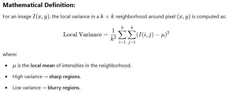
Local Variance Method

The Local Variance method measures local intensity variations, assuming that sharp images exhibit higher contrast and variance compared to blurry ones. It computes the variance of pixel intensities within a neighborhood, making it useful for detecting focus in an image.

Pros:

Simple and Fast – Computationally efficient and easy to implement.
Effective for High-Contrast Images – Works well when images have strong edges and variations in intensity.
Noise-Robust (to Some Extent) – Less affected by small variations in pixel intensity compared to gradient-based methods.

Cons:

Fails on Low-Contrast Images – If the image has uniform intensity (e.g., blurry but high brightness), it may incorrectly assign a high score.
Sensitive to Illumination Changes – Uneven lighting can influence variance, leading to inaccurate sharpness evaluation.
Not the Best for Autofocus – Inconsistent performance when compared with gradient-based methods.

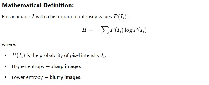
Entropy-Based Focus Measure

The entropy-based focus measure quantifies image sharpness by analyzing the distribution of intensity values. Sharp images contain more detailed information and have a higher entropy value, while blurry images tend to have a more uniform intensity distribution and lower entropy.

Pros:

Works Well for Texture-Rich Images – Best suited for images with a lot of detailed textures and patterns.
Resistant to Small Amounts of Noise – Can still give reliable results in mildly noisy images.
Good for Low-Contrast Situations – Performs better than variance-based methods when contrast is low.

Cons:

Computationally Expensive – Requires histogram computation and logarithmic calculations, making it slower than variance or gradient methods.
Sensitive to Noise in High-Frequency Regions – If an image has excessive noise, entropy may incorrectly identify it as “sharp” due to increased randomness.
Not Ideal for Edge-Based Sharpness Detection – Doesn’t work well in images where sharpness is mainly defined by edges rather than textures.

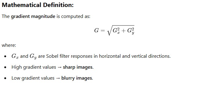
Tenengrad (Sobel Gradient-Based) Focus Measure

The Tenengrad method evaluates image sharpness based on edge strength. It relies on the Sobel operator, which detects intensity variations in both horizontal and vertical directions. The assumption is that sharper images contain stronger edges, leading to higher gradient values.

Pros:

Strong Edge Detection – Works well for sharpness detection in images with strong edges.
Resistant to Illumination Changes – More robust compared to variance-based methods.
Good for Autofocus Applications – Commonly used in autofocus systems due to its effectiveness in detecting sharp transitions.

Cons:

Sensitive to Noise – Small noise variations can create strong gradients, leading to false sharpness detection.
Fails in Texture-Rich Low-Edge Images – If an image is highly detailed but lacks clear edges, the method may underestimate sharpness.
Directional Sensitivity – If a structure in the image aligns with the gradient direction, it may produce misleading results.

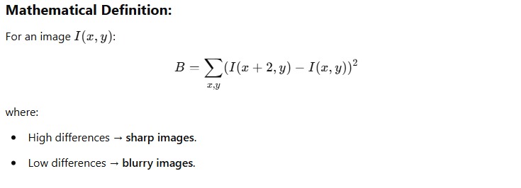
Brenner Gradient Focus Measure

The Brenner Gradient method evaluates image sharpness based on pixel intensity differences between adjacent pixels. The assumption is that a sharper image has larger intensity variations, resulting in higher focus scores.

Pros:

Very Simple and Fast – Faster than Sobel or Laplacian methods since it only uses pixel-wise differences.
Effective for Edge-Based Sharpness – Works well for detecting sharp changes in pixel intensity.
Good for Defocused Images – Performs better than variance-based methods in blurry images.

Cons:

Not Very Robust – Can be unreliable in low-contrast or texture-rich images.
Sensitive to Noise – May falsely classify noise patterns as sharp features.
Limited Use in General Applications – Works well for specific autofocus scenarios but not for all types of images.

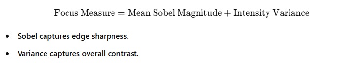
Sobel + Variance Combination

This method enhances focus measurement by combining two approaches:

1. Sobel Gradient – Measures edge strength in an image by computing intensity changes in both horizontal and vertical directions.
2. Local Intensity Variance – Determines sharpness by analyzing the variation in pixel intensities, assuming sharper images have higher contrast and variance.

By combining these two measures, this method provides a more robust focus evaluation, capturing both edge sharpness and local intensity variations.

Pros:

Balances Edges and Intensity Information – More robust than using Sobel or variance alone.
Handles Both Edge-Based and Texture-Based Sharpness – Effective for various types of images.
More Reliable in Autofocus Applications – Reduces misclassification due to noise.

Cons:

Computationally More Expensive – Slightly slower due to multiple calculations.
Still Somewhat Sensitive to Noise – While more robust than individual methods, it may still struggle in extremely noisy images.
Requires Proper Parameter Tuning – Performance depends on selecting an appropriate Sobel kernel size and variance threshold.

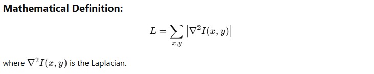
Laplacian-Based Method

This method uses the Laplacian operator, a second-order derivative filter, to detect edges in an image. It measures the variance of the Laplacian response, assuming that sharper images have stronger edge responses with higher variance, while blurry images have smoother transitions and lower variance.

Pros:

Captures High-Frequency Sharpness – Stronger in detecting fine details and subtle edges.
Good for General Autofocus Applications – Used in many image-processing and microscopy autofocus systems.
Less Affected by Global Illumination Changes – More stable under varying lighting conditions compared to variance-based methods.

Cons:

Very Sensitive to Noise – More prone to amplifying noise compared to Sobel-based methods.
Computationally Expensive – Slightly slower than simpler operators like variance or Brenner gradient.
Edge Overemphasis Can Cause False Positives – May incorrectly classify an image as “sharp” if there is too much edge contrast (e.g., due to noise or artifacts).

Implementation of Each Method

To evaluate different focus measures, we apply each method to every frame in a video, compute its focus score, and select the sharpest frame. The code remains the same across different methods, with only the focus measure function being replaced.

The process involves:

• Reading the video frames one by one.
• Computing the focus score using the selected focus measure.
• Storing the frames and their scores for later comparison.
• Selecting the frame with the highest focus score as the sharpest frame.
• Print out the best frame number and its focus score.
• Displaying the best frame to visually verify the effectiveness of each method.

Python Syntax

import cv2
import numpy as np

videoPath = "C:/Users/ssabb/Desktop/opencv_courses/articles/data/autofocus1.mp4"
cap = cv2.VideoCapture(videoPath)
focus_scores = []
frames = []

# Include the function for focus measures here
# def compute_focus_measure(image):

#     Implement the focus measure function here (e.g., Tenengrad, Brenner, etc.)
if cap.isOpened():
    print("Video file successfully retrieved")
else:
    print("Video file wasn't retrieved properly")
while True:
    ret, frame = cap.read()
    if ret:
        focus_scores.append(compute_focus_measure(frame))  # Replace with actual function
        frames.append(frame)
    else:
        print("Frame not read")
        break
cap.release()

# Find the best-focused frame
best_score_index = np.argmax(focus_scores)
best_frame = frames[best_score_index]
print(f"Best frame index: {best_score_index} with score {focus_scores[best_score_index]}")

# Get the original dimensions
original_height, original_width = best_frame.shape[:2]
new_width = 600
aspect_ratio = new_width / original_width
new_height = int(original_height * aspect_ratio)  # Compute height based on aspect ratio

# Resize the image
resized_image = cv2.resize(best_frame, (new_width, new_height))

# Display the best frame
cv2.imshow("Best Frame", resized_image)
cv2.waitKey(0)
cv2.destroyAllWindows()

Replace compute_focus_measure(image) with the appropriate function for each method (e.g., compute_tenengrad(image), compute_entropy(image), etc.).

Local Variance Method

Python Syntax

# Function to compute Local Variance focus measure
def compute_local_variance(image, ksize=5):
    gray = cv2.cvtColor(image, cv2.COLOR_BGR2GRAY)
    mean = cv2.blur(gray, (ksize, ksize))
    squared_mean = cv2.blur(gray**2, (ksize, ksize))
    variance = squared_mean - (mean**2)
    return np.mean(variance)

Entropy-Based Focus Measure

Python Syntax

from skimage.measure import shannon_entropy
import cv2

def compute_entropy(image):
    gray = cv2.cvtColor(image, cv2.COLOR_BGR2GRAY)
    return shannon_entropy(gray)

Tenengrad (Sobel Gradient-Based) Focus Measure

Python Syntax

def compute_tenengrad(image):
    gray = cv2.cvtColor(image, cv2.COLOR_BGR2GRAY)  # Convert to grayscale
    sobel_x = cv2.Sobel(gray, cv2.CV_64F, 1, 0, ksize=3)  # Sobel filter in X direction
    sobel_y = cv2.Sobel(gray, cv2.CV_64F, 0, 1, ksize=3)  # Sobel filter in Y direction
    tenengrad = np.sqrt(sobel_x**2 + sobel_y**2)  # Compute gradient magnitude
    return np.mean(tenengrad)  # Return mean gradient magnitude as focus score

Brenner Gradient Focus Measure

Python Syntax

def compute_brenner_gradient(image):
    gray = cv2.cvtColor(image, cv2.COLOR_BGR2GRAY)  # Convert to grayscale
    shifted = np.roll(gray, -2, axis=1)  # Shift by 2 pixels horizontally
    diff = (gray - shifted) ** 2  # Compute squared difference
    return np.sum(diff)  # Sum all differences as the focus measure

Sobel + Variance Combination

Python Syntax

def compute_sobel_variance(image):
    gray = cv2.cvtColor(image, cv2.COLOR_BGR2GRAY)  # Convert to grayscale
    sobel_x = cv2.Sobel(gray, cv2.CV_64F, 1, 0, ksize=3)  # Sobel X gradient
    sobel_y = cv2.Sobel(gray, cv2.CV_64F, 0, 1, ksize=3)  # Sobel Y gradient
    sobel_magnitude = np.sqrt(sobel_x**2 + sobel_y**2)  # Compute gradient magnitude
    variance = np.var(gray)  # Compute variance of pixel intensities
    return np.mean(sobel_magnitude) + variance  # Combine Sobel and variance

Laplacian-Based Method

Python Syntax

def compute_laplacian(image):
    gray = cv2.cvtColor(image, cv2.COLOR_BGR2GRAY)  # Convert to grayscale
    laplacian = cv2.Laplacian(gray, cv2.CV_64F)  # Apply Laplacian filter
    return np.var(laplacian)  # Compute variance of Laplacian

Output

The sharpest frames detected by different focus operators are displayed sequentially.

Performance Comparison

We analyze and compare the performance of various focus operators based on their ability to identify the best-focused frame.

Method	Performance
Local Variance	Selected highly blurred frames. The method is unreliable because it confuses smooth regions with sharpness.
Entropy-Based	Selected blurred frames. Struggles in low-texture regions where entropy is low, regardless of sharpness.
Brenner Gradient	Performed better but still had some blurring. Measures pixel differences but doesn’t fully capture edges.
Sobel + Variance	Identified sharp frames accurately. Gradient strength combined with variance improves detection.
Tenengrad (Sobel)	Found perfect sharp frames. Gradient-based methods effectively detect strong edges.
Laplacian-Based	Also detected perfect sharp frames. Variance of second derivative captures high-frequency details.

Key Takeaways

• Local Variance and Entropy failed because they rely on intensity statistics that do not strongly correlate with focus.
• Brenner Gradient performed moderately well but was slightly less effective than gradient-based methods.
• Sobel + Variance, Tenengrad, and Laplacian were the best methods, as they effectively captured edge sharpness.

Thus, for selecting the sharpest frame, Tenengrad, Laplacian, and Sobel + Variance should be the preferred choices.

Summary

In this article, we explored various focus measurement operators to identify the sharpest frame in a video sequence. We implemented and analyzed methods such as Local Variance, Entropy, Tenengrad (Sobel Gradient), Brenner Gradient, Sobel + Variance, and Laplacian-based approach. Through experimentation, we observed that Local Variance and Entropy struggled to accurately detect sharp frames, often selecting blurry ones. The Brenner Gradient performed better but was not perfect, while Sobel + Variance, Tenengrad, and Laplacian-based methods consistently identified the sharpest frame with high accuracy.

This study highlights the importance of selecting an appropriate focus measure for autofocus applications in imaging systems.

References

In this article, we explored various focus measurement operators based on the techniques presented in the following research papers. However, we have intentionally left out two focus methods for you to explore and experiment with, allowing for further investigation into autofocus performance.

• Nayar, S. K., & Nakagawa, Y. (1992). Shape from Focus. Proceedings of the IEEE Conference on Computer Vision and Pattern Recognition (CVPR). Link
• Santos, A. M., Costa, E. S., & do Amaral, C. F. (2002). Diatom Autofocusing in Brightfield Microscopy: A Comparative Study. Proceedings of the 16th International Conference on Pattern Recognition. Link

You can explore additional methods in Analysis of Focus Measure Operators in Shape-from-Focus and experiment with their implementation to evaluate their effectiveness in different scenarios.